Minimum Working Examples

create_mwe	Create a minimal (parameterized) working example using tessif's model.
create_fpwe	Create a fully parameterized working example using tessif's model.
emission_objective	Create a minimal working example using tessif's model optimizing it for costs and keeping the total emissions below an emission objective.
create_connected_es	Create a minimal working example using tessif's model connecting to seperate energy systems using a tessif.model.components.Connector object.
create_chp	Create a minimal working example using tessif's model optimizing it for costs to demonstrate a chp application.
create_variable_chp	Same as create_chp() but with two chps that use additional functionality from tessif's tessif.model.components.CHP class.
create_storage_example	Create a small energy system utilizing a storage.
create_expansion_plan_example	Create a small energy system utilizing two emisison free and expandable sources, as well as an emitting one.
create_simple_transformer_grid_es	Create a simplified grid energy system for testing.
create_time_varying_efficiency_transformer	Create a small es having a transformer with varying efficiency.

Meaningful working Examples

create_self_similar_energy_system	Create a self-similar energy system.
_create_minimal_es_unit	Create a minimal self simular energy system unit.

Full Fledged Use Case Wrappers

create_hhes	Create a model of Hamburg's energy system using tessif's model.
create_grid_es	Create a model of a generic grid style energy system using tessif's model.
create_component_es	Create a model of a generic component based energy system using tessif's model.
create_grid_kp_es	Create a model of a generic grid style energy system using tessif's model.
create_grid_cs_es	Create a model of a generic grid style energy system using tessif's model.
create_grid_cp_es	Create a model of a generic grid style energy system using tessif's model.
create_grid_ts_es	Create a model of a generic grid style energy system using tessif's model.
create_grid_tp_es	Create a model of a generic grid style energy system using tessif's model.
create_transcne_es	Create the TransCnE system model scenarios combinations.

py - hardcoded

py_hard is a tessif module for giving examples on how to create a tessif energy system.

It collects minimum working examples, meaningful working examples and full-fledged use case wrappers for common scenarios.

tessif.examples.data.tsf.py_hard.create_mwe(directory=None, filename=None)

Create a minimal (parameterized) working example using tessif's model.

Creates a simple energy system simulation to potentially store it on disc inside directory as filename.

Parameters:

• directory (str, default=None) –

  String representing of the path the created energy system is dumped to. Passed to dump() .

  Will be joined with filename.

  If set to None (default) tessif.frused.paths.write_dir/tsf will be the chosen directory.

• filename (str, default=None) –

  dump() the energy system using this name.

  If set to None (default) filename will be mwe.tsf.

Returns:

es – Tessif energy system.

Return type:

tessif.model.energy_system.AbstractEnergySystem

See also

Minimum Working Example

Examples

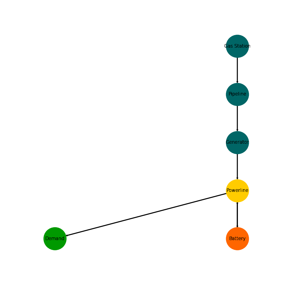
Use create_mwe() to quickly access a tessif energy system to use for doctesting, or trying out this framework’s utilities.

>>> import tessif.examples.data.tsf.py_hard as tsf_py
>>> es = tsf_py.create_mwe()

>>> for node in es.nodes:
...     print(node.uid.name)
Pipeline
Powerline
Gas Station
Demand
Generator
Battery

Visualize the energy system for better understanding what the output means:

>>> import matplotlib.pyplot as plt
>>> import tessif.visualize.nxgrph as nxv
>>> grph = es.to_nxgrph()
>>> drawing_data = nxv.draw_graph(
...     grph,
...     node_color={
...         'Gas Station': '#006666',
...         'Pipeline': '#006666',
...         'Generator': '#006666',
...         'Powerline': '#ffcc00',
...         'Battery': '#ff6600',
...         'Demand': '#009900',
...     },
... )
>>> # plt.show()  # commented out for simpler doctesting

tessif.examples.data.tsf.py_hard.create_fpwe(directory=None, filename=None)

Create a fully parameterized working example using tessif's model.

Creates a simple energy system simulation to potentially store it on disc inside directory as filename.

Parameters:

• directory (str, default=None) –

  String representing of the path the created energy system is dumped to. Passed to dump() .

  Will be joined with filename.

  If set to None (default) tessif.frused.paths.write_dir/tsf will be the chosen directory.

• filename (str, default=None) –

  dump() the energy system using this name.

  If set to None (default) filename will be fpwe.tsf.

Returns:

es – Tessif energy system.

Return type:

tessif.model.energy_system.AbstractEnergySystem

References

Fully Parameterized Working Example - For a step by step explanation on creating this energy system.

Fully Parameterized Working Example (Detailed) - For simulating and comparing the fpwe using different supported models.

Examples

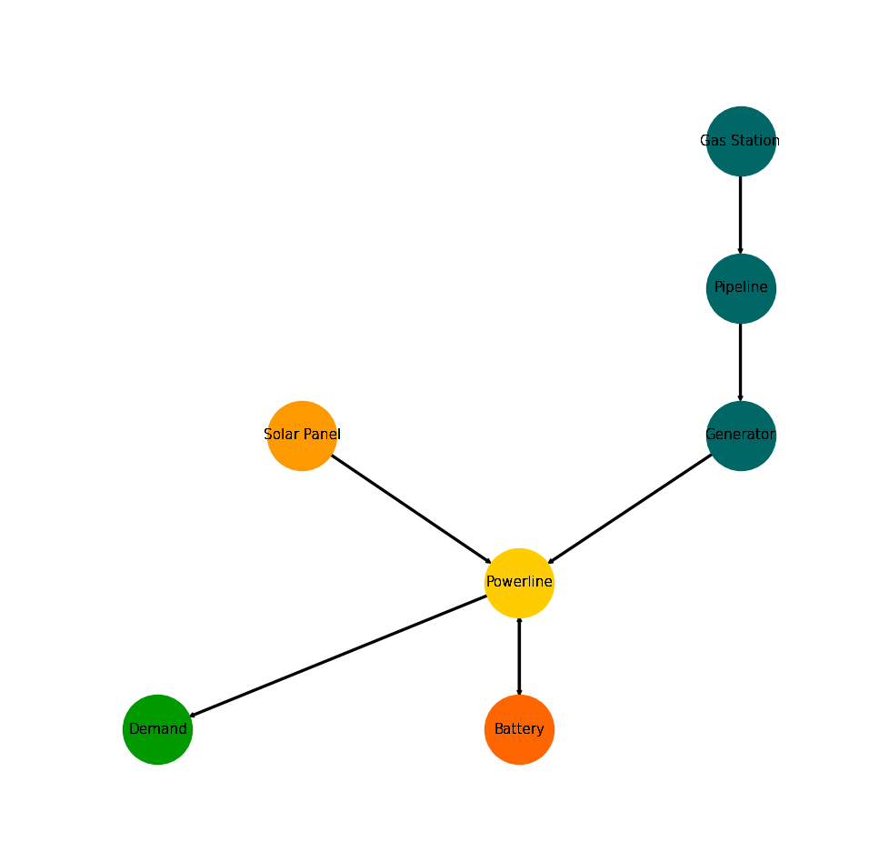
Use create_fpwe() to quickly access a tessif energy system to use for doctesting, or trying out this framework’s utilities.

>>> import tessif.examples.data.tsf.py_hard as tsf_py
>>> es = tsf_py.create_fpwe()

>>> for node in es.nodes:
...     print(node.uid.name)
Pipeline
Powerline
Gas Station
Solar Panel
Demand
Generator
Battery

Visualize the energy system for better understanding what the output means:

>>> import matplotlib.pyplot as plt
>>> import tessif.visualize.nxgrph as nxv
>>> grph = es.to_nxgrph()
>>> drawing_data = nxv.draw_graph(
...     grph,
...     node_color={
...         'Solar Panel': '#ff9900',
...         'Gas Station': '#006666',
...         'Pipeline': '#006666',
...         'Generator': '#006666',
...         'Powerline': '#ffcc00',
...         'Battery': '#ff6600',
...         'Demand': '#009900',
...     },
... )
>>> # plt.show()  # commented out for simpler doctesting

tessif.examples.data.tsf.py_hard.emission_objective(directory=None, filename=None)

Create a minimal working example using tessif's model optimizing it for costs and keeping the total emissions below an emission objective.

Creates a simple energy system simulation to potentially store it on disc inside directory as filename.

Parameters:

• directory (str, default=None) –

  String representing of the path the created energy system is dumped to. Passed to dump() .

  Will be joined with filename.

  If set to None (default) tessif.frused.paths.write_dir/tsf will be the chosen directory.

• filename (str, default=None) –

  dump() the energy system using this name.

  If set to None (default) filename will be emission_objective.tsf.

Returns:

es – Tessif energy system.

Return type:

tessif.model.energy_system.AbstractEnergySystem

References

Minimum Working Example - For a step by step explanation on how to create a Tessif energy system.

Emission Objective (Brief) - For simulating and comparing this energy system using different supported models.

Secondary Objectives - For a detailed description on how to constrain values like co2 emissions.

Examples

Use emission_objective() to quickly access a tessif energy system to use for doctesting or trying out this framework’s utilities.

>>> import tessif.examples.data.tsf.py_hard as tsf_py
>>> es = tsf_py.emission_objective()
>>> print(es.global_constraints['emissions'])
60

Transform the energy system to i.e. oemof, to see if the constraint holds:

>>> import tessif.transform.es2es.omf as tessif_to_oemof
>>> oemof_es = tessif_to_oemof.transform(es)
>>> print(oemof_es.global_constraints['emissions'])
60

Optmize the energy system to see the constraint’s consequences:

>>> import tessif.simulate as simulate
>>> optimized_oemof_es = simulate.omf_from_es(oemof_es, solver='cbc')

>>> import tessif.transform.es2mapping.omf as oemof_results
>>> resultier = oemof_results.LoadResultier(optimized_oemof_es)

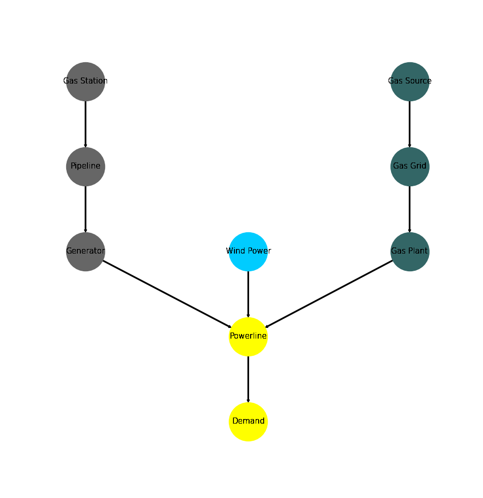
>>> # Generator costs/emissions are 2/1 unit respectively
>>> # Wind Power costs/emissions are 4/0 units respectively
>>> print(resultier.node_load['Powerline'])
Powerline            Gas Plant  Generator  Wind Power  Demand
1990-07-13 00:00:00       -5.0  -0.000000   -5.000000    10.0
1990-07-13 01:00:00       -5.0  -0.000000   -5.000000    10.0
1990-07-13 02:00:00       -5.0  -0.000000   -5.000000    10.0
1990-07-13 03:00:00       -5.0  -0.507246   -4.492754    10.0

Visualize the energy system for better understanding what the output means:

>>> import matplotlib.pyplot as plt
>>> import tessif.visualize.nxgrph as nxv
>>> grph = es.to_nxgrph()
>>> drawing_data = nxv.draw_graph(
...     grph,
...     node_color={
...         'Wind Power': '#00ccff',
...         'Gas Source': '#336666',
...         'Gas Grid': '#336666',
...         'Gas Plant': '#336666',
...         'Gas Station': '#666666',
...         'Pipeline': '#666666',
...         'Generator': '#666666',
...         'Powerline': 'yellow',
...         'Demand': 'yellow',
...     },
... )
>>> # plt.show()  # commented out for simpler doctesting

tessif.examples.data.tsf.py_hard.create_connected_es(directory=None, filename=None)

Create a minimal working example using tessif's model connecting to seperate energy systems using a tessif.model.components.Connector object. Effectively creating a transs hipment problem.

Creates a simple energy system simulation to potentially store it on disc inside directory as filename.

Parameters:

• directory (str, default=None) –

  String representing of the path the created energy system is dumped to. Passed to dump() .

  Will be joined with filename.

  If set to None (default) tessif.frused.paths.write_dir/tsf will be the chosen directory.

• filename (str, default=None) –

  dump() the energy system using this name.

  If set to None (default) filename will be connected_es.tsf.

Returns:

es – Tessif energy system.

Return type:

tessif.model.energy_system.AbstractEnergySystem

References

Minimum Working Example - For a step by step explanation on how to create a Tessif energy system.

Transshipment Problem Example (Brief) - For simulating and comparing this energy system using different supported models.

tessif.model.energy_system.AbstractEnergySystem.connect() - For the built-in mehtod of tessif’s energy systems.

Estimating Computational Resources - For a comprehensive example on how to connect energy systems and how this can be used to measure computational scalability.

Examples

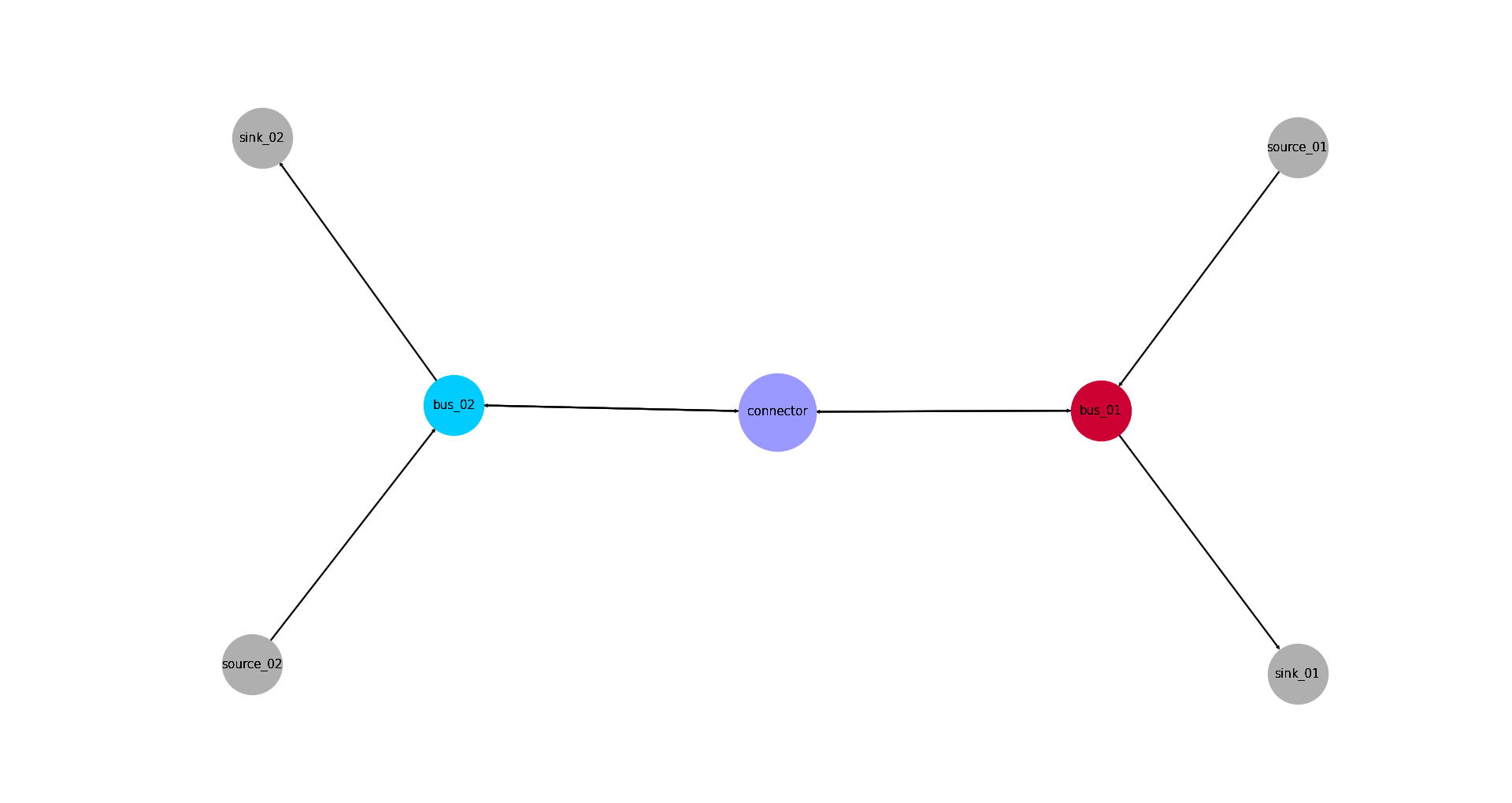
Use create_connected_es() to quickly access a tessif energy system to use for doctesting or trying out this framework’s utilities:

>>> import tessif.examples.data.tsf.py_hard as coded_examples
>>> es = coded_examples.create_connected_es()
>>> for connector in es.connectors:
...     print(connector.conversions)
{('bus-01', 'bus-02'): 0.9, ('bus-02', 'bus-01'): 0.8}

Transform the energy system to i.e. oemof, to see if conversion factors remain:

>>> import tessif.transform.es2es.omf as tessif_to_oemof
>>> oemof_es = tessif_to_oemof.transform(es)
>>> for node in oemof_es.nodes:
...     if node.label.name == 'connector':
...        for bus_tuple, factor in node.conversion_factors.items():
...            print('({}, {}): {}'.format(
...                bus_tuple[0], bus_tuple[1], factor[0]))
(bus-01, bus-02): 0.9
(bus-02, bus-01): 0.8

Optmize the energy system to see the transhipment problem:

>>> import tessif.simulate as simulate
>>> optimized_oemof_es = simulate.omf_from_es(oemof_es, solver='cbc')

>>> import tessif.transform.es2mapping.omf as oemof_results
>>> resultier = oemof_results.LoadResultier(optimized_oemof_es)

>>> print(resultier.node_load['connector'])
connector              bus-01  bus-02  bus-01  bus-02
1990-07-13 00:00:00 -5.555556   -0.00     0.0     5.0
1990-07-13 01:00:00 -0.000000   -6.25     5.0     0.0
1990-07-13 02:00:00 -0.000000   -0.00     0.0     0.0

>>> print(resultier.node_load['bus-01'])
bus-01               connector  source-01  connector  sink-01
1990-07-13 00:00:00       -0.0  -5.555556   5.555556      0.0
1990-07-13 01:00:00       -5.0 -10.000000   0.000000     15.0
1990-07-13 02:00:00       -0.0 -10.000000   0.000000     10.0

>>> print(resultier.node_load['bus-02'])
bus-02               connector  source-02  connector  sink-02
1990-07-13 00:00:00       -5.0     -10.00       0.00     15.0
1990-07-13 01:00:00       -0.0      -6.25       6.25      0.0
1990-07-13 02:00:00       -0.0     -10.00       0.00     10.0

Visualize the energy system for better understanding what the output means:

>>> import matplotlib.pyplot as plt
>>> import tessif.visualize.nxgrph as nxv
>>> grph = es.to_nxgrph()
>>> drawing_data = nxv.draw_graph(
...     grph,
...     node_color={'connector': '#9999ff',
...                 'bus-01': '#cc0033',
...                 'bus-02': '#00ccff'},
...     node_size={'connector': 5000},
...     layout='neato')
>>> # plt.show()  # commented out for simpler doctesting

tessif.examples.data.tsf.py_hard.create_storage_example(directory=None, filename=None)

Create a small energy system utilizing a storage.

Creates a simple energy system simulation to potentially store it on disc inside directory as filename.

Parameters:

• directory (str, default=None) –

  String representing of the path the created energy system is dumped to. Passed to dump() .

  Will be joined with filename.

  If set to None (default) tessif.frused.paths.write_dir/tsf will be the chosen directory.

• filename (str, default=None) –

  dump() the energy system using this name.

  If set to None (default) filename will be storage_example.tsf.

Returns:

es – Tessif energy system.

Return type:

tessif.model.energy_system.AbstractEnergySystem

Warning

In this example the installed capacity is set to 0, but expandable (A common use case). Most, if not any, of the supported models however, use capacity specific values for idle losses and initial as well as final soc constraints.

Given the initial capacity is 0, this problem is solved by setting the initial soc as well as the idle losses to 0, if necessary.

To avoid this caveat, set the inital capacity to a small value and adjust initial soc and idle changes accordingly. This might involve some trial and error.

References

Minimum Working Example - For a step by step explanation on how to create a Tessif energy system.

Storage Example (Brief) - For simulating and comparing this energy system using different supported models.

Examples

Use create_storage_example() to quickly access a tessif energy system to use for doctesting or trying out this framework’s utilities.

>>> import tessif.examples.data.tsf.py_hard as coded_examples
>>> tsf_es = coded_examples.create_storage_example()

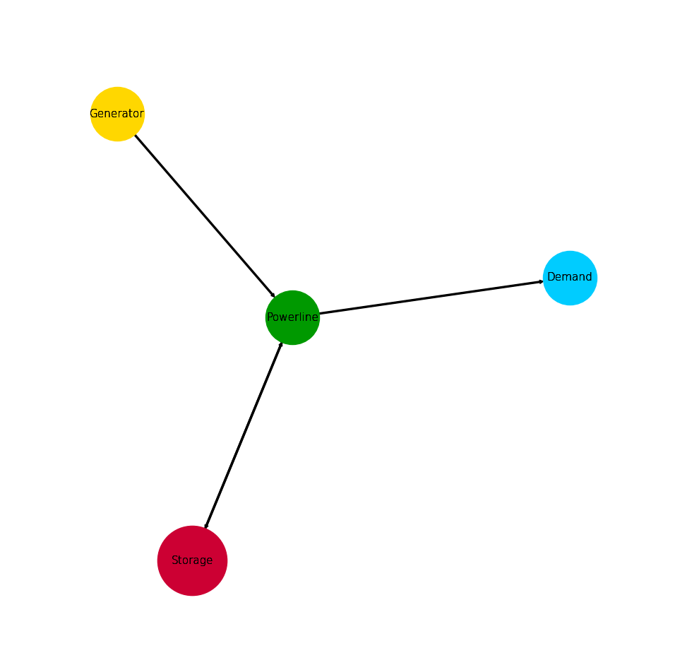
>>> for node in tsf_es.nodes:
...     print(node.uid.name)
Powerline
Generator
Demand
Storage

Transform the tessif energy system into oemof and pypsa:

>>> # Import the model transformation utilities:
>>> from tessif.transform.es2es import (
...     ppsa as tsf2pypsa,
...     omf as tsf2omf,
... )

>>> # Do the transformation:
>>> oemof_es = tsf2omf.transform(tsf_es)
>>> pypsa_es = tsf2pypsa.transform(tsf_es)

Do some examplary checks on the flow conversions:

>>> # oemof:
>>> for node in oemof_es.nodes:
...     if node.label.name == 'Storage':
...         print(node.inflow_conversion_factor[0])
...         print(node.outflow_conversion_factor[0])
0.9
0.9

>>> # pypsa:
>>> print(pypsa_es.storage_units['efficiency_store']['Storage'])
0.9
>>> print(pypsa_es.storage_units['efficiency_dispatch']['Storage'])
0.9

Simulate the transformed energy system:

>>> # Import the simulation utility:
>>> import tessif.simulate

>>> # Optimize the energy systems:
>>> optimized_oemof_es = tessif.simulate.omf_from_es(oemof_es)
>>> optimized_pypsa_es = tessif.simulate.ppsa_from_es(pypsa_es)

Do some post processing:

>>> # Import the post-processing utilities:
>>> from tessif.transform.es2mapping import (
...     ppsa as post_process_pypsa,
...     omf as post_process_oemof,
... )

>>> # Conduct the post-processing:
>>> oemof_load_results = post_process_oemof.LoadResultier(
...     optimized_oemof_es)
>>> pypsa_load_results = post_process_pypsa.LoadResultier(
...     optimized_pypsa_es)

To see the load results:

>>> # oemof:
>>> oemof_loads = post_process_oemof.LoadResultier(optimized_oemof_es)
>>> print(oemof_loads.node_load['Powerline'])
Powerline            Generator  Storage  Demand  Storage
1990-07-13 00:00:00      -19.0     -0.0    10.0      9.0
1990-07-13 01:00:00      -19.0     -0.0    10.0      9.0
1990-07-13 02:00:00      -19.0     -0.0     7.0     12.0
1990-07-13 03:00:00       -0.0    -10.0    10.0      0.0
1990-07-13 04:00:00       -0.0    -10.0    10.0      0.0

>>> # pypsa:
>>> pypsa_loads = post_process_pypsa.LoadResultier(optimized_pypsa_es)
>>> print(pypsa_loads.node_load['Powerline'])
Powerline            Generator  Storage  Demand  Storage
1990-07-13 00:00:00      -19.0     -0.0    10.0      9.0
1990-07-13 01:00:00      -19.0     -0.0    10.0      9.0
1990-07-13 02:00:00      -19.0     -0.0     7.0     12.0
1990-07-13 03:00:00       -0.0    -10.0    10.0      0.0
1990-07-13 04:00:00       -0.0    -10.0    10.0      0.0

And to check the state of charge results:

>>> # oemof:
>>> oemof_socs = post_process_oemof.StorageResultier(optimized_oemof_es)
>>> print(oemof_socs.node_soc['Storage'])
1990-07-13 00:00:00     8.100000
1990-07-13 01:00:00    16.200000
1990-07-13 02:00:00    27.000000
1990-07-13 03:00:00    15.888889
1990-07-13 04:00:00     4.777778
Freq: H, Name: Storage, dtype: float64

>>> # pypsa:
>>> pypsa_socs = post_process_pypsa.StorageResultier(optimized_pypsa_es)
>>> print(pypsa_socs.node_soc['Storage'])
1990-07-13 00:00:00     8.100000
1990-07-13 01:00:00    16.200000
1990-07-13 02:00:00    27.000000
1990-07-13 03:00:00    15.888889
1990-07-13 04:00:00     4.777778
Freq: H, Name: Storage, dtype: float64

Visualize the energy system for better understanding what the output means:

>>> import matplotlib.pyplot as plt
>>> import tessif.visualize.nxgrph as nxv
>>> grph = tsf_es.to_nxgrph()
>>> drawing_data = nxv.draw_graph(
...     grph,
...     node_color={'Powerline': '#009900',
...                 'Storage': '#cc0033',
...                 'Demand': '#00ccff',
...                 'Generator': '#ffD700',},
...     node_size={'Storage': 5000},
...     layout='neato')
>>> # plt.show()  # commented out for simpler doctesting

tessif.examples.data.tsf.py_hard.create_storage_fixed_ratio_expansion_example(directory=None, filename=None)

Create a small energy system utilizing an expandable storage with a fixed capacity to outflow ratio.

Creates a simple energy system simulation to potentially store it on disc inside directory as filename.

Parameters:

• directory (str, default=None) –

  String representing of the path the created energy system is dumped to. Passed to dump() .

  Will be joined with filename.

  If set to None (default) tessif.frused.paths.write_dir/tsf will be the chosen directory.

• filename (str, default=None) –

  dump() the energy system using this name.

  If set to None (default) filename will be storage_fixed_ratio_example.tsf.

Returns:

es – Tessif energy system.

Return type:

tessif.model.energy_system.AbstractEnergySystem

Warning

In this example the installed capacity is set to 1, but expandable. The flow rate to 0.1. By enabling both expandables (capacity and flow rate) as well as fixing their ratios the installed capacity result will be much higher than needed. Or in other words, the flow rate will determine the amount of installed capacity.

References

Minimum Working Example - For a step by step explanation on how to create a Tessif energy system.

Storage Example (Brief) - For simulating and comparing this energy system using different supported models.

Examples

Use create_storage_fixed_ratio_expansion_example() to quickly access a tessif energy system to use for doctesting, or trying out this framework’s utilities.

>>> import tessif.examples.data.tsf.py_hard as coded_examples
>>> tsf_es = coded_examples.create_storage_fixed_ratio_expansion_example()

>>> for node in tsf_es.nodes:
...     print(node.uid.name)
Powerline
Generator
Demand
Storage

Transform the tessif energy system into oemof and pypsa:

>>> # Import the model transformation utilities:
>>> from tessif.transform.es2es import (
...     ppsa as tsf2pypsa,
...     omf as tsf2omf,
... )

>>> # Do the transformation:
>>> oemof_es = tsf2omf.transform(tsf_es)
>>> pypsa_es = tsf2pypsa.transform(tsf_es)

Do some examplary checks on the flow conversions:

>>> # oemof:
>>> for node in oemof_es.nodes:
...     if node.label.name == 'Storage':
...         print(node.inflow_conversion_factor[0])
...         print(node.outflow_conversion_factor[0])
0.95
0.89

>>> # pypsa:
>>> print(pypsa_es.storage_units['efficiency_store']['Storage'])
0.95
>>> print(pypsa_es.storage_units['efficiency_dispatch']['Storage'])
0.89

Simulate the transformed energy system:

>>> # Import the simulation utility:
>>> import tessif.simulate

>>> # Optimize the energy systems:
>>> optimized_oemof_es = tessif.simulate.omf_from_es(oemof_es)
>>> optimized_pypsa_es = tessif.simulate.ppsa_from_es(pypsa_es)

Do some post processing:

>>> # Import the post-processing utilities:
>>> from tessif.transform.es2mapping import (
...     ppsa as post_process_pypsa,
...     omf as post_process_oemof,
... )

>>> # Conduct the post-processing:
>>> oemof_load_results = post_process_oemof.LoadResultier(
...     optimized_oemof_es)
>>> pypsa_load_results = post_process_pypsa.LoadResultier(
...     optimized_pypsa_es)

Check if the load results are the same as in the example above:

>>> # oemof:
>>> oemof_loads = post_process_oemof.LoadResultier(optimized_oemof_es)
>>> print(oemof_loads.node_load['Powerline'])
Powerline            Generator  Storage  Demand  Storage
1990-07-13 00:00:00      -19.0     -0.0    10.0      9.0
1990-07-13 01:00:00      -19.0     -0.0    10.0      9.0
1990-07-13 02:00:00      -19.0     -0.0     7.0     12.0
1990-07-13 03:00:00       -0.0    -10.0    10.0      0.0
1990-07-13 04:00:00       -0.0    -10.0    10.0      0.0

>>> # pypsa:
>>> pypsa_loads = post_process_pypsa.LoadResultier(optimized_pypsa_es)
>>> print(pypsa_loads.node_load['Powerline'])
Powerline            Generator  Storage  Demand  Storage
1990-07-13 00:00:00      -19.0     -0.0    10.0      9.0
1990-07-13 01:00:00      -19.0     -0.0    10.0      9.0
1990-07-13 02:00:00      -19.0     -0.0     7.0     12.0
1990-07-13 03:00:00       -0.0    -10.0    10.0      0.0
1990-07-13 04:00:00       -0.0    -10.0    10.0      0.0

Check the installed capacity:

>>> # oemof:
>>> oemof_capacities = post_process_oemof.CapacityResultier(
...     optimized_oemof_es)
>>> print(oemof_capacities.node_installed_capacity['Storage'])
120.0

>>> # pypsa:
>>> pypsa_capacities = post_process_pypsa.CapacityResultier(
...     optimized_pypsa_es)
>>> print(pypsa_capacities.node_installed_capacity['Storage'])
120.0

The integrated global results or high priority resutls:

>>> # oemof:
>>> oemof_hps = post_process_oemof.IntegratedGlobalResultier(
...     optimized_oemof_es)
>>> for key, result in oemof_hps.global_results.items():
...     if 'emissions' not in key:
...          print(f'{key}: {result}')
costs (sim): 258.0
opex (ppcd): 20.0
capex (ppcd): 238.0

>>> # pypsa:
>>> pypsa_hps = post_process_pypsa.IntegratedGlobalResultier(
...     optimized_pypsa_es)
>>> for key, result in pypsa_hps.global_results.items():
...     if 'emissions' not in key:
...          print(f'{key}: {result}')
costs (sim): 258.0
opex (ppcd): 20.0
capex (ppcd): 238.0

And to check the state of charge results:

>>> # oemof:
>>> oemof_socs = post_process_oemof.StorageResultier(optimized_oemof_es)
>>> print(oemof_socs.node_soc['Storage'])
1990-07-13 00:00:00     8.550000
1990-07-13 01:00:00    17.100000
1990-07-13 02:00:00    28.500000
1990-07-13 03:00:00    17.264045
1990-07-13 04:00:00     6.028090
Freq: H, Name: Storage, dtype: float64

>>> # pypsa:
>>> pypsa_socs = post_process_pypsa.StorageResultier(optimized_pypsa_es)
>>> print(pypsa_socs.node_soc['Storage'])
1990-07-13 00:00:00     8.550000
1990-07-13 01:00:00    17.100000
1990-07-13 02:00:00    28.500000
1990-07-13 03:00:00    17.264045
1990-07-13 04:00:00     6.028090
Freq: H, Name: Storage, dtype: float64

Visualize the energy system for better understanding what the output means:

>>> import matplotlib.pyplot as plt
>>> import tessif.visualize.nxgrph as nxv
>>> grph = tsf_es.to_nxgrph()
>>> drawing_data = nxv.draw_graph(
...     grph,
...     node_color={'Powerline': '#009900',
...                 'Storage': '#cc0033',
...                 'Demand': '#00ccff',
...                 'Generator': '#ffD700',},
...     node_size={'Storage': 5000},
...     layout='neato')
>>> # plt.show()  # commented out for simpler doctesting

Reparameterize the storage component usinng one of tessif’s hooks, to unbind capacity and flow rate expansion:

>>> from tessif.frused.hooks.tsf import reparameterize_components
>>> reparameterized_es = reparameterize_components(
...     es=tsf_es,
...     components={
...         'Storage': {
...             'fixed_expansion_ratios': {'electricity': False},
...         },
...     },
... )

Redo the transformations and simulations:

>>> # Transformation:
>>> oemof_es = tsf2omf.transform(reparameterized_es)
>>> pypsa_es = tsf2pypsa.transform(reparameterized_es)

>>> # Optimization/Simulation:
>>> optimized_oemof_es = tessif.simulate.omf_from_es(oemof_es)
>>> optimized_pypsa_es = tessif.simulate.ppsa_from_es(pypsa_es)

Recheck installed capacities socs and loads:

Installed capacity:

>>> # oemof:
>>> oemof_capacities = post_process_oemof.CapacityResultier(
...     optimized_oemof_es)
>>> print(oemof_capacities.node_installed_capacity['Storage'])
28.5

>>> # pypsa:
>>> pypsa_capacities = post_process_pypsa.CapacityResultier(
...     optimized_pypsa_es)
>>> print(pypsa_capacities.node_installed_capacity['Storage'])
120.0

Note

Note how oemof is able to unbind these values, whereas pypsa is not.

Integrated global results or high priority resutls:

>>> # oemof:
>>> oemof_hps = post_process_oemof.IntegratedGlobalResultier(
...     optimized_oemof_es)
>>> for key, result in oemof_hps.global_results.items():
...     if 'emissions' not in key:
...          print(f'{key}: {result}')
costs (sim): 75.0
opex (ppcd): 20.0
capex (ppcd): 55.0

>>> # pypsa:
>>> pypsa_hps = post_process_pypsa.IntegratedGlobalResultier(
...     optimized_pypsa_es)
>>> for key, result in pypsa_hps.global_results.items():
...     if 'emissions' not in key:
...          print(f'{key}: {result}')
costs (sim): 258.0
opex (ppcd): 20.0
capex (ppcd): 238.0

Note

Note how PyPSA still calculates higher capex for the storage expansion, since cpacity and power ratio are fixed.

State of charge results:

>>> # oemof:
>>> oemof_socs = post_process_oemof.StorageResultier(optimized_oemof_es)
>>> print(oemof_socs.node_soc['Storage'])
1990-07-13 00:00:00     8.550000
1990-07-13 01:00:00    17.100000
1990-07-13 02:00:00    28.500000
1990-07-13 03:00:00    17.264045
1990-07-13 04:00:00     6.028090
Freq: H, Name: Storage, dtype: float64

>>> # pypsa:
>>> pypsa_socs = post_process_pypsa.StorageResultier(optimized_pypsa_es)
>>> print(pypsa_socs.node_soc['Storage'])
1990-07-13 00:00:00     8.550000
1990-07-13 01:00:00    17.100000
1990-07-13 02:00:00    28.500000
1990-07-13 03:00:00    17.264045
1990-07-13 04:00:00     6.028090
Freq: H, Name: Storage, dtype: float64

Loads:

>>> # oemof:
>>> oemof_loads = post_process_oemof.LoadResultier(optimized_oemof_es)
>>> print(oemof_loads.node_load['Powerline'])
Powerline            Generator  Storage  Demand  Storage
1990-07-13 00:00:00      -19.0     -0.0    10.0      9.0
1990-07-13 01:00:00      -19.0     -0.0    10.0      9.0
1990-07-13 02:00:00      -19.0     -0.0     7.0     12.0
1990-07-13 03:00:00       -0.0    -10.0    10.0      0.0
1990-07-13 04:00:00       -0.0    -10.0    10.0      0.0

>>> # pypsa:
>>> pypsa_loads = post_process_pypsa.LoadResultier(optimized_pypsa_es)
>>> print(pypsa_loads.node_load['Powerline'])
Powerline            Generator  Storage  Demand  Storage
1990-07-13 00:00:00      -19.0     -0.0    10.0      9.0
1990-07-13 01:00:00      -19.0     -0.0    10.0      9.0
1990-07-13 02:00:00      -19.0     -0.0     7.0     12.0
1990-07-13 03:00:00       -0.0    -10.0    10.0      0.0
1990-07-13 04:00:00       -0.0    -10.0    10.0      0.0

tessif.examples.data.tsf.py_hard.create_expansion_plan_example(directory=None, filename=None)

Create a small energy system utilizing two emisison free and expandable sources, as well as an emitting one.

Creates a simple energy system simulation to potentially store it on disc inside directory as filename.

Parameters:

• directory (str, default=None) –

  String representing of the path the created energy system is dumped to. Passed to dump() .

  Will be joined with filename.

  If set to None (default) tessif.frused.paths.write_dir/tsf will be the chosen directory.

• filename (str, default=None) –

  dump() the energy system using this name.

  If set to None (default) filename will be expp.tsf.

Returns:

es – Tessif energy system.

Return type:

tessif.model.energy_system.AbstractEnergySystem

References

Minimum Working Example - For a step by step explanation on how to create a Tessif energy system.

Expansion Example (Brief) - For simulating and comparing this energy system using different supported models.

Component Focused Model Scenario Combinations, - For a comprehensive example on a reference energy system to analyze and compare commitment optimization among models.

Examples

Use create_expansion_plan_example() to quickly access a tessif energy system to use for doctesting, or trying out this framework’s utilities.

(For a step by step explanation see Minimum Working Example):

>>> import tessif.examples.data.tsf.py_hard as tsf_py
>>> es = tsf_py.create_expansion_plan_example()

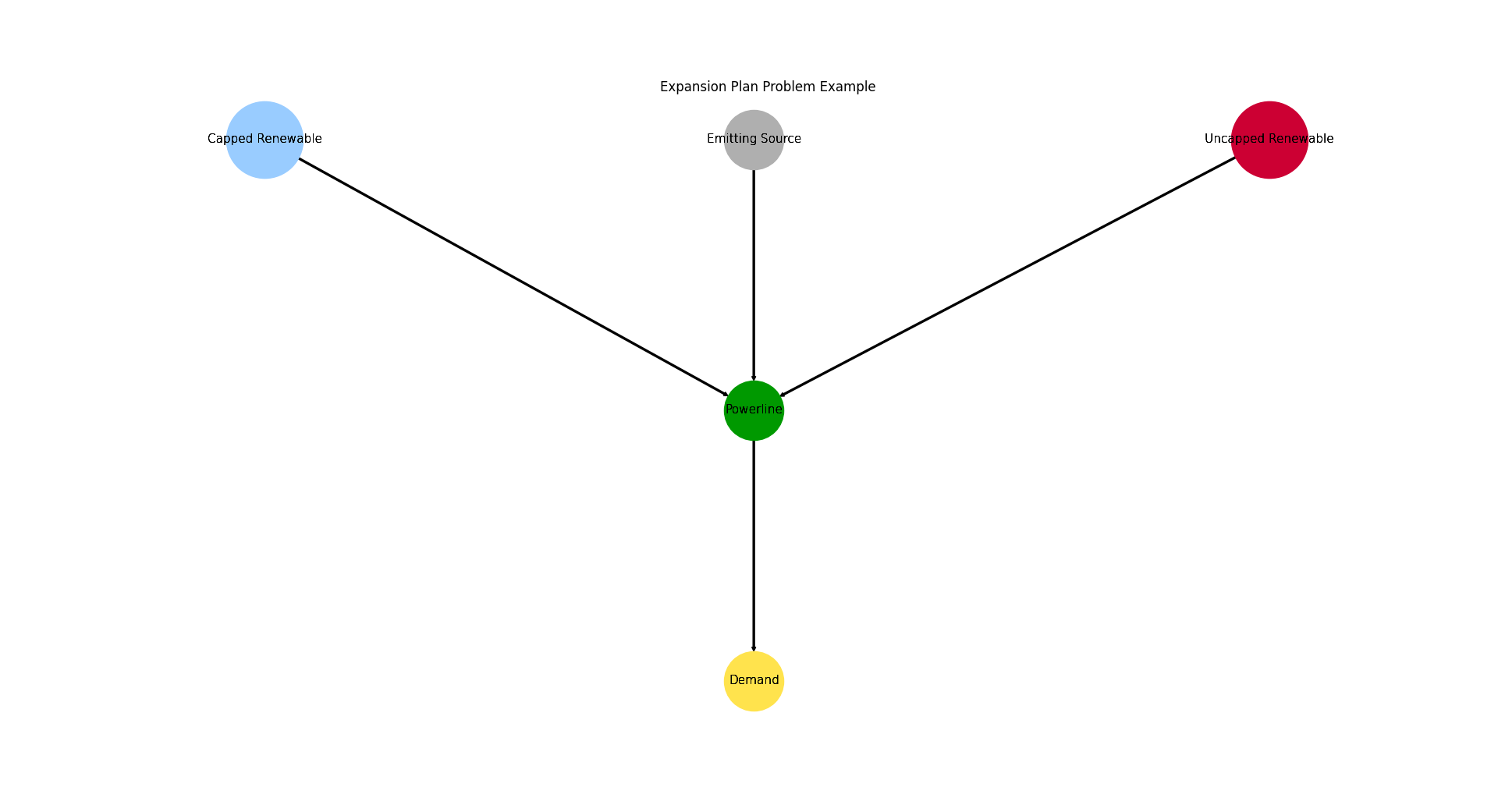
>>> for node in es.nodes:
...     print(str(node.uid))
Powerline
Emitting Source
Capped Renewable
Uncapped Renewable
Demand

Visualize the energy system for better understanding what the output means:

>>> import matplotlib.pyplot as plt
>>> import tessif.visualize.nxgrph as nxv
>>> grph = es.to_nxgrph()
>>> drawing_data = nxv.draw_graph(
...     grph,
...     node_color={'Powerline': '#009900',
...                 'Emitting Source': '#cc0033',
...                 'Demand': '#00ccff',
...                 'Capped Renewable': '#ffD700',
...                 'Uncapped Renewable': '#ffD700',},
...     node_size={'Powerline': 5000},
...     layout='dot')
>>> # plt.show()  # commented out for simpler doctesting

tessif.examples.data.tsf.py_hard.create_zero_costs_es(directory=None, filename=None)

Create a small energy system having to costs alocated to commitment and expansion, but a low emission consttaint.

Interesting about this example is the fact that there are many possible solutions, so solver ambiguity might be observed using this es. This energy system also serves as a method of validation for the post-processing capabilities, to handle 0 costs in case of scaling results to maximum occuring costs.

Creates a simple energy system simulation to potentially store it on disc inside directory as filename.

Parameters:

• directory (str, default=None) –

  String representing of the path the created energy system is dumped to. Passed to dump() .

  Will be joined with filename.

  If set to None (default) tessif.frused.paths.write_dir/tsf will be the chosen directory.

• filename (str, default=None) –

  dump() the energy system using this name.

  If set to None (default) filename will be expp.tsf.

Returns:

es – Tessif energy system.

Return type:

tessif.model.energy_system.AbstractEnergySystem

References

Minimum Working Example - For a step by step explanation on how to create a Tessif energy system.

Examples

Use create_zero_costs_es() to quickly access a tessif energy system to use for doctesting, or trying out this framework’s utilities.

(For a step by step explanation see Minimum Working Example):

>>> import tessif.examples.data.tsf.py_hard as tsf_py
>>> es = tsf_py.create_zero_costs_es()

>>> for node in es.nodes:
...     print(str(node.uid))
Powerline
Emitting Source
Capped Renewable
Uncapped Renewable
Demand

Visualize the energy system for better understanding what the output means:

>>> import matplotlib.pyplot as plt
>>> import tessif.visualize.nxgrph as nxv
>>> grph = es.to_nxgrph()
>>> drawing_data = nxv.draw_graph(
...     grph,
...     node_color={'Powerline': '#009900',
...                 'Emitting Source': '#cc0033',
...                 'Demand': '#00ccff',
...                 'Capped Renewable': '#ffD700',
...                 'Uncapped Renewable': '#ffD700',},
...     node_size={'Powerline': 5000},
...     layout='dot')
>>> # plt.show()  # commented out for simpler doctesting

tessif.examples.data.tsf.py_hard.create_self_similar_energy_system(N=1, timeframe=None, unit='minimal', **kwargs)

Create a self-similar energy system.

This energy system is obtained by repeating its unit N times. The singular units are connected to each other through their central bus. Meaning the central bus of energy system N is connected to the central bus of energy system N-1 via a Connector object.

Parameters:

• N (int) – Number of units the self similar energy system consists of.

• timeframe (pandas.DatetimeIndex) –

  Datetime index representing the evaluated timeframe. Explicitly stating:

  • initial datatime (0th element of the pandas.DatetimeIndex)

  • number of time steps (length of pandas.DatetimeIndex)

  • temporal resolution (pandas.DatetimeIndex.freq)

  For example:

  idx = pd.DatetimeIndex(
      data=pd.date_range(
          '2016-01-01 00:00:00', periods=11, freq='H'))
  

• unit (str) –

  Specify which of tessif’s hardcoded examples should be used as unit of the self similar energy system.

  Currently available are:

  • ’minimal’:

    Uses _create_minimal_es_unit() which is the smallest unit available.

  • ’component’:

    Uses _create_component_es_unit() which is based on create_component_es().

  • ’grid’:

    Uses _create_grid_es_unit() which is based on create_transcne_es().

  • ’hamburg’:

    Uses _create_hhes_unit() which is based on create_hhes_unit().

• kwargs – Are passed to the _create_[…]_unit() function.

Examples

Create a self similar energy system out of N=2 minimum self similar energy system units:

>>> from tessif.frused.paths import example_dir
>>> import os
>>> storage_path = os.path.join(example_dir, 'data', 'tsf',)

>>> import tessif.examples.data.tsf.py_hard as coded_examples
>>> sses = coded_examples.create_self_similar_energy_system(N=2)

# Create an image using AbstractEnergySystem.to_nxgrph() and # tessif.visualize.nxgrph

tessif.examples.data.tsf.py_hard.create_chp(directory=None, filename=None)

Create a minimal working example using tessif's model optimizing it for costs to demonstrate a chp application.

Creates a simple energy system simulation to potentially store it on disc inside directory as filename.

Parameters:

• directory (str, default=None) –

  String representing of the path the created energy system is dumped to. Passed to dump() .

  Will be joined with filename.

  If set to None (default) tessif.frused.paths.write_dir/tsf will be the chosen directory.

• filename (str, default=None) –

  dump() the energy system using this name.

  If set to None (default) filename will be chp.tsf.

Returns:

es – Tessif energy system.

Return type:

tessif.model.energy_system.AbstractEnergySystem

References

Minimum Working Example - For a step by step explanation on how to create a Tessif energy system.

Combined Heat and Power Example (Brief) - For simulating and comparing this energy system using different supported models.

Examples

Use create_chp() to quickly access a tessif energy system to use for doctesting or trying out this framework’s utilities.

(For a step by step explanation see Minimum Working Example):

>>> import tessif.examples.data.tsf.py_hard as tsf_py
>>> es = tsf_py.create_chp()

>>> for node in es.nodes:
...     print(node.uid)
Gas Grid
Powerline
Heat Grid
Gas Source
Backup Power
Backup Heat
Power Demand
Heat Demand
CHP

tessif.examples.data.tsf.py_hard.create_variable_chp(directory=None, filename=None)

Same as create_chp() but with two chps that use additional functionality from tessif’s tessif.model.components.CHP class.

Creates a simple energy system simulation to potentially store it on disc inside directory as filename.

Parameters:

• directory (str, default=None) –

  String representing of the path the created energy system is dumped to. Passed to dump() .

  Will be joined with filename.

  If set to None (default) tessif.frused.paths.write_dir/tsf will be the chosen directory.

• filename (str, default=None) –

  dump() the energy system using this name.

  If set to None (default) filename will be chp.tsf.

Returns:

es – Tessif energy system.

Return type:

tessif.model.energy_system.AbstractEnergySystem

References

Minimum Working Example - For a step by step explanation on how to create a Tessif energy system.

Combined Heat and Power Example (Brief) - For simulating and comparing this energy system using different supported models.

Examples

Use create_chp() to quickly access a tessif energy system to use for doctesting or trying out this framework’s utilities.

(For a step by step explanation see Minimum Working Example):

>>> import tessif.examples.data.tsf.py_hard as tsf_py
>>> es = tsf_py.create_variable_chp()

>>> for node in es.nodes:
...     print(node.uid)
Gas Grid
Powerline
Heat Grid
CHP1
CHP2
Gas Source
Backup Power
Backup Heat
Power Demand
Heat Demand

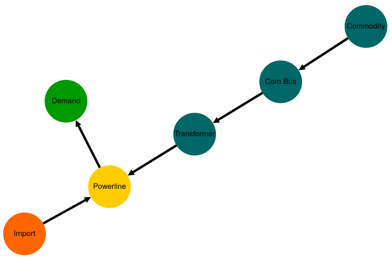
tessif.examples.data.tsf.py_hard.create_time_varying_efficiency_transformer()

Create a small es having a transformer with varying efficiency.

Returns:

Tessif minimum working example energy system.

Return type:

tessif.model.energy_system.AbstractEnergySystem

Example

Visualize the energy system for better understanding what the output means:

>>> import tessif.visualize.dcgrph as dcv  # nopep8

>>> app = dcv.draw_generic_graph(
...     energy_system=create_time_varying_efficiency_transformer(),
...     color_group={
...         'Transformer': '#006666',
...         'Commodity': '#006666',
...         'Com Bus': '#006666',
...         'Powerline': '#ffcc00',
...         'Import': '#ff6600',
...         'Demand': '#009900',
...      },
...  )

>>>  # Serve interactive drawing to http://127.0.0.1:8050/
>>>  # app.run_server(debug=False)

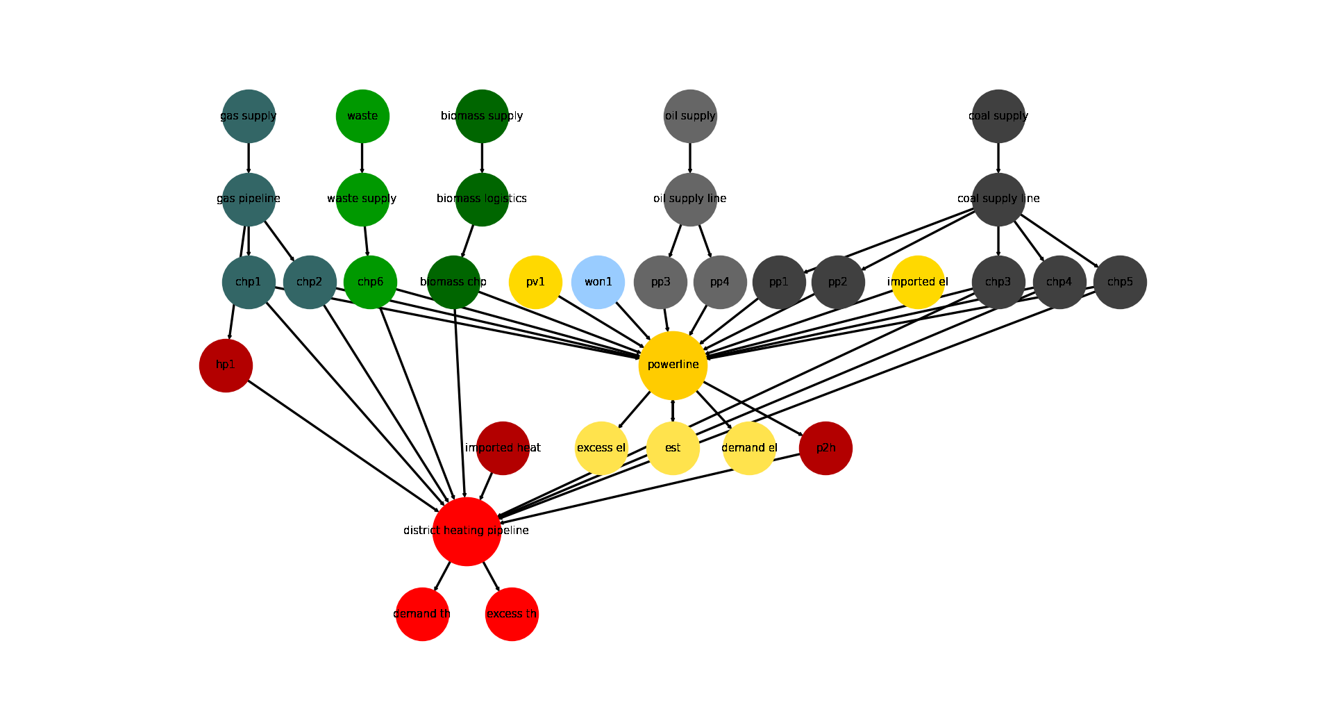
tessif.examples.data.tsf.py_hard.create_hhes(periods=24, directory=None, filename=None)

Create a model of Hamburg’s energy system using tessif's model.

Parameters:

• periods (int, default=24) – Number of time steps of the evaluated timeframe (one time step is one hour)

• directory (str, default=None) –

  String representing of the path the created energy system is dumped to. Passed to dump() .

  Will be joined with filename.

  If set to None (default) tessif.frused.paths.write_dir/tsf will be the chosen directory.

• filename (str, default=None) –

  dump() the energy system using this name.

  If set to None (default) filename will be hhes.tsf.

Returns:

es – Tessif energy system.

Return type:

tessif.model.energy_system.AbstractEnergySystem

References

Minimum Working Example - For a step by step explanation on how to create a Tessif energy system.

Hamburg Energy System Example (Brief) - For simulating and comparing this energy system using different supported models.

Examples

Use create_hhes() to quickly access a tessif energy system to use for doctesting, or trying out this framework’s utilities.

>>> import tessif.examples.data.tsf.py_hard as tsf_py
>>> es = tsf_py.create_hhes()

>>> for node in es.nodes:
...     print(node.uid)
coal supply line
gas pipeline
oil supply line
waste supply
powerline
district heating pipeline
biomass logistics
gas supply
coal supply
oil supply
waste
pv1
won1
biomass supply
imported el
imported heat
demand el
demand th
excess el
excess th
chp1
chp2
chp3
chp4
chp5
chp6
pp1
pp2
pp3
pp4
hp1
p2h
biomass chp
est

Visualize the energy system for better understanding what the output means:

>>> import matplotlib.pyplot as plt
>>> import tessif.visualize.nxgrph as nxv
>>> grph = es.to_nxgrph()
>>> drawing_data = nxv.draw_graph(
...     grph,
...     node_color={
...         'coal supply': '#404040',
...         'coal supply line': '#404040',
...         'pp1': '#404040',
...         'pp2': '#404040',
...         'chp3': '#404040',
...         'chp4': '#404040',
...         'chp5': '#404040',
...         'hp1': '#b30000',
...         'imported heat': '#b30000',
...         'district heating pipeline': 'Red',
...         'demand th': 'Red',
...         'excess th': 'Red',
...         'p2h': '#b30000',
...         'bm1': '#006600',
...         'won1': '#99ccff',
...         'gas supply': '#336666',
...         'gas pipeline': '#336666',
...         'chp1': '#336666',
...         'chp2': '#336666',
...         'waste': '#009900',
...         'waste supply': '#009900',
...         'chp6': '#009900',
...         'oil supply': '#666666',
...         'oil supply line': '#666666',
...         'pp3': '#666666',
...         'pp4': '#666666',
...         'pv1': '#ffd900',
...         'imported el': '#ffd900',
...         'demand el': '#ffe34d',
...         'excess el': '#ffe34d',
...         'est': '#ffe34d',
...         'powerline': '#ffcc00',
...     },
...     node_size={
...         'powerline': 5000,
...         'district heating pipeline': 5000
...     },
...     layout='dot',
... )
>>> # plt.show()  # commented out for simpler doctesting

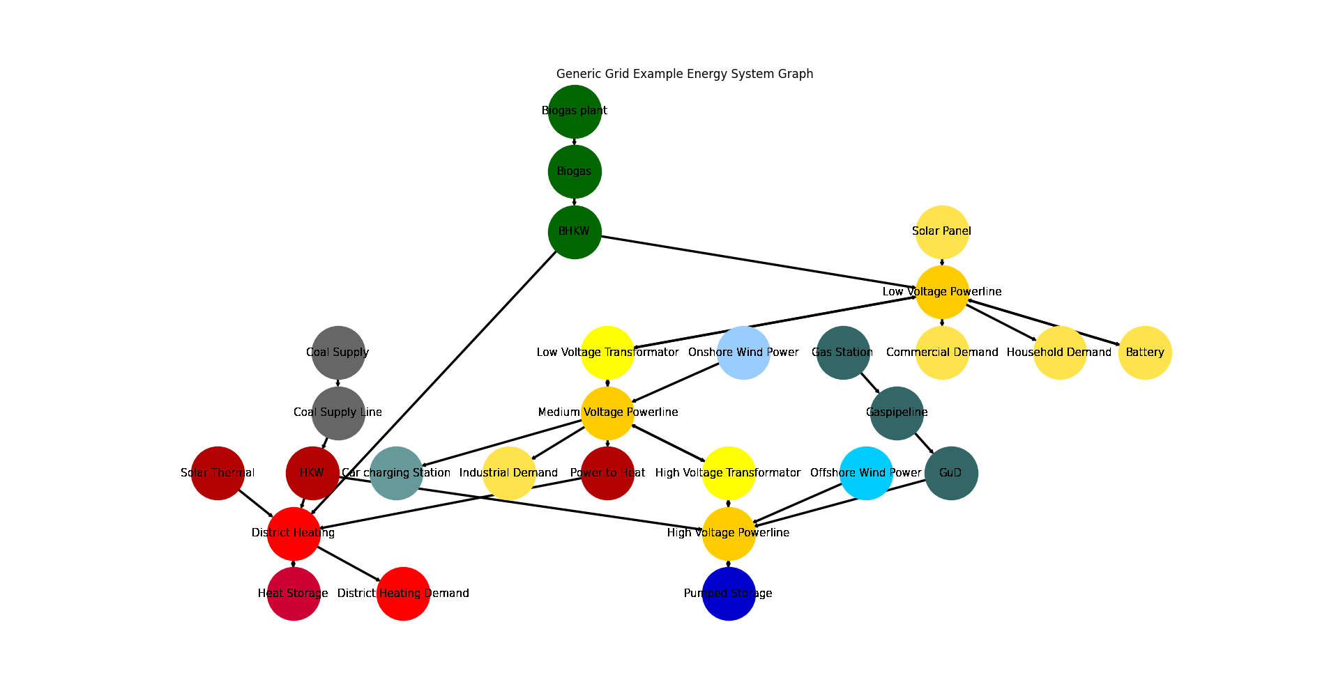
tessif.examples.data.tsf.py_hard.create_grid_es(periods=3, directory=None, filename=None)

Create a model of a generic grid style energy system using tessif's model.

Parameters:

• periods (int, default=3) – Number of time steps of the evaluated timeframe (one time step is one hour)

• directory (str, default=None) –

  String representing of the path the created energy system is dumped to. Passed to dump() .

  Will be joined with filename.

  If set to None (default) tessif.frused.paths.write_dir/tsf will be the chosen directory.

• filename (str, default=None) –

  dump() the energy system using this name.

  If set to None (default) filename will be grid_es.tsf.

Returns:

es – Tessif energy system.

Return type:

tessif.model.energy_system.AbstractEnergySystem

References

Minimum Working Example - For a step by step explanation on how to create a Tessif energy system.

Generic Grid Example (Brief) - For simulating and comparing this energy system using different supported models.

Grid Focused Model Scenario Combinations, - For a comprehensive example on a reference energy system to analyze and compare commitment optimization respecting among models.

Examples

Use create_grid_es() to quickly access a tessif energy system to use for doctesting, or trying out this framework’s utilities.

>>> import tessif.examples.data.tsf.py_hard as tsf_py
>>> es = tsf_py.create_grid_es()

>>> for node in es.nodes:
...     print(node.uid)
Gaspipeline
Low Voltage Powerline
District Heating
Medium Voltage Powerline
High Voltage Powerline
Coal Supply Line
Biogas
Solar Panel
Gas Station
Onshore Wind Power
Offshore Wind Power
Coal Supply
Solar Thermal
Biogas plant
Household Demand
Commercial Demand
District Heating Demand
Industrial Demand
Car charging Station
BHKW
Power to Heat
GuD
HKW
Battery
Heat Storage
Pumped Storage
Low Voltage Transformator
High Voltage Transformator

Visualize the energy system for better understanding what the output means:

>>> import matplotlib.pyplot as plt
>>> import tessif.visualize.nxgrph as nxv
>>> grph = es.to_nxgrph()
>>> drawing_data = nxv.draw_graph(
...     grph,
...     node_color={
...         'Coal Supply': '#666666',
...         'Coal Supply Line': '#666666',
...         'HKW': '#b30000',
...         'Solar Thermal': '#b30000',
...         'Heat Storage': '#cc0033',
...         'District Heating': 'Red',
...         'District Heating Demand': 'Red',
...         'Power to Heat': '#b30000',
...         'Biogas plant': '#006600',
...         'Biogas': '#006600',
...         'BHKW': '#006600',
...         'Onshore Wind Power': '#99ccff',
...         'Offshore Wind Power': '#00ccff',
...         'Gas Station': '#336666',
...         'Gaspipeline': '#336666',
...         'GuD': '#336666',
...         'Solar Panel': '#ffe34d',
...         'Commercial Demand': '#ffe34d',
...         'Household Demand': '#ffe34d',
...         'Industrial Demand': '#ffe34d',
...         'Battery': '#ffe34d',
...         'Car charging Station': '#669999',
...         'Low Voltage Powerline': '#ffcc00',
...         'Medium Voltage Powerline': '#ffcc00',
...         'High Voltage Powerline': '#ffcc00',
...         'High Voltage Transformator': 'yellow',
...         'Low Voltage Transformator': 'yellow',
...         'Pumped Storage': '#0000cc',
...     },
...     title='Generic Grid Example Energy System Graph',
... )
>>> # plt.show()  # commented out for simpler doctesting

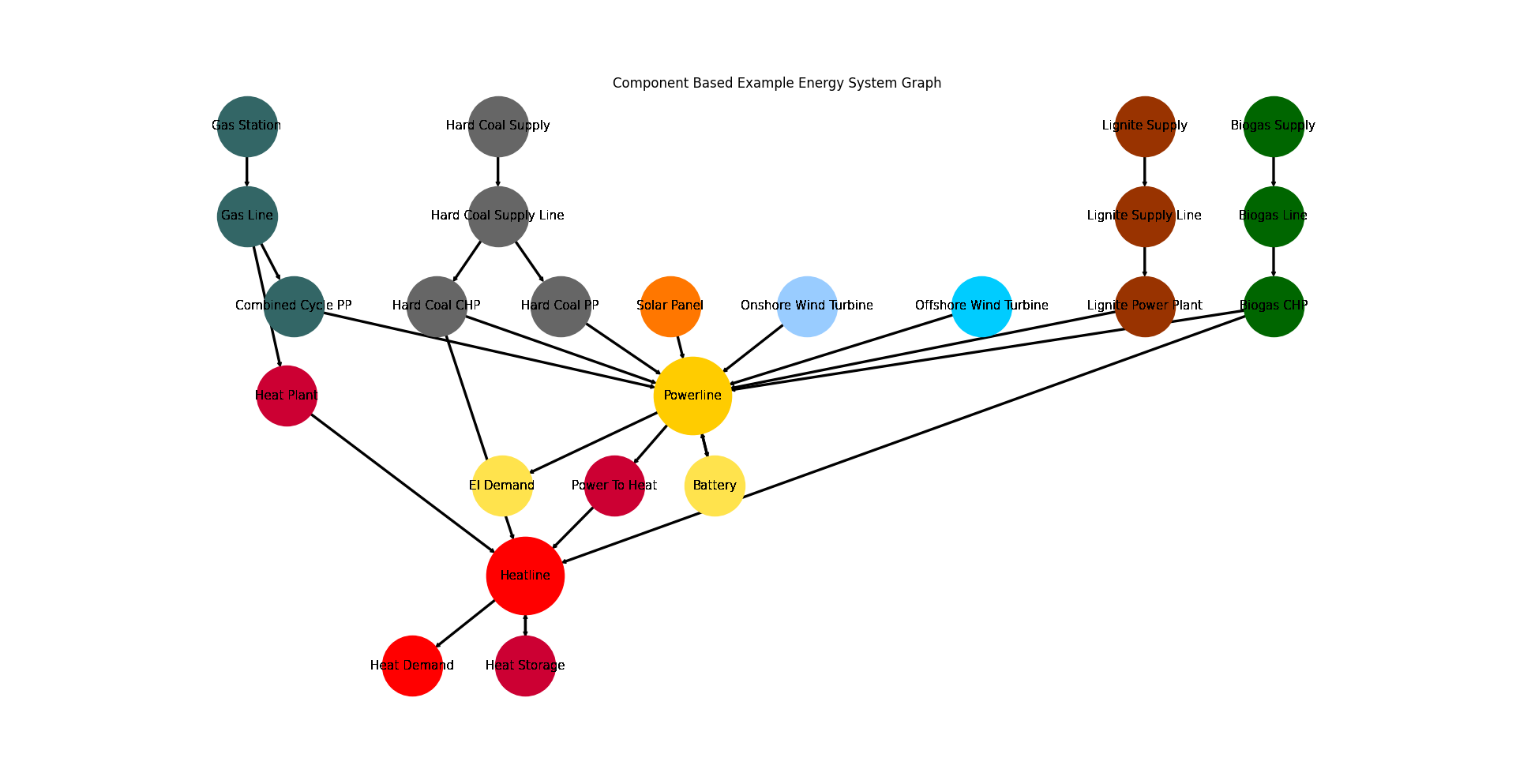
tessif.examples.data.tsf.py_hard.create_component_es(expansion_problem=False, periods=3, directory=None, filename=None)

Create a model of a generic component based energy system using tessif's model.

Parameters:

• expansion_problem (bool, default=False) – Boolean which states whether a commitment problem (False) or expansion problem (True) is to be solved

• periods (int, default=3) – Number of time steps of the evaluated timeframe (one time step is one hour)

• directory (str, default=None) –

  String representing of the path the created energy system is dumped to. Passed to dump() .

  Will be joined with filename.

  If set to None (default) tessif.frused.paths.write_dir/tsf will be the chosen directory.

• filename (str, default=None) –

  dump() the energy system using this name.

  If set to None (default) filename will be component_es.tsf.

Returns:

es – Tessif energy system.

Return type:

tessif.model.energy_system.AbstractEnergySystem

References

Minimum Working Example - For a step by step explanation on how to create a Tessif energy system.

Component Focused Model Scenario Combinations, - For a comprehensive example on a reference energy system to analyze and compare commitment optimization respecting among models.

Examples

Use create_component_es() to quickly access a tessif energy system to use for doctesting, or trying out this framework’s utilities.

>>> import tessif.examples.data.tsf.py_hard as tsf_py
>>> es = tsf_py.create_component_es()

>>> for node in es.nodes:
...     print(node.uid)
Gas Line
Powerline
Hard Coal Supply Line
Lignite Supply Line
Biogas Line
Heatline
Gas Station
Solar Panel
Onshore Wind Turbine
Hard Coal Supply
Lignite Supply
Offshore Wind Turbine
Biogas Supply
El Demand
Heat Demand
Combined Cycle PP
Hard Coal PP
Lignite Power Plant
Biogas CHP
Heat Plant
Power To Heat
Hard Coal CHP
Battery
Heat Storage

Visualize the energy system for better understanding what the output means:

>>> import matplotlib.pyplot as plt
>>> import tessif.visualize.nxgrph as nxv
>>> grph = es.to_nxgrph()
>>> drawing_data = nxv.draw_graph(
...     grph,
...     node_color={
...        'Hard Coal Supply': '#666666',
...        'Hard Coal Supply Line': '#666666',
...        'Hard Coal PP': '#666666',
...        'Hard Coal CHP': '#666666',
...        'Solar Panel': '#FF7700',
...        'Heat Storage': '#cc0033',
...        'Heat Demand': 'Red',
...        'Heat Plant': '#cc0033',
...        'Heatline': 'Red',
...        'Power To Heat': '#cc0033',
...        'Biogas CHP': '#006600',
...        'Biogas Line': '#006600',
...        'Biogas Supply': '#006600',
...        'Onshore Wind Turbine': '#99ccff',
...        'Offshore Wind Turbine': '#00ccff',
...        'Gas Station': '#336666',
...        'Gas Line': '#336666',
...        'Combined Cycle PP': '#336666',
...        'El Demand': '#ffe34d',
...        'Battery': '#ffe34d',
...        'Powerline': '#ffcc00',
...        'Lignite Supply': '#993300',
...        'Lignite Supply Line': '#993300',
...        'Lignite Power Plant': '#993300',
...      },
...     node_size={
...        'Powerline': 5000,
...        'Heatline': 5000
...    },
...      title='Component Based Example Energy System Graph',
... )
>>> # plt.show()  # commented out for simpler doctesting

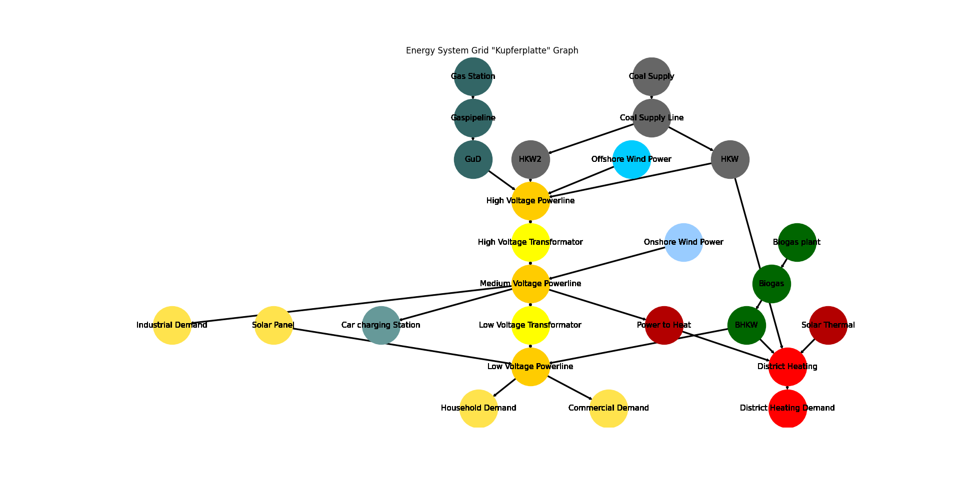
tessif.examples.data.tsf.py_hard.create_grid_kp_es(periods=24, directory=None, filename=None)

Create a model of a generic grid style energy system using tessif's model.

Parameters:

• periods (int, default=24) – Number of time steps of the evaluated timeframe (one time step is one hour)

• directory (str, default=None) –

  String representing of the path the created energy system is dumped to. Passed to dump() .

  Will be joined with filename.

  If set to None (default) tessif.frused.paths.write_dir/tsf will be the chosen directory.

• filename (str, default=None) –

  dump() the energy system using this name.

  If set to None (default) filename will be grid_es_KP.tsf.

Returns:

es – Tessif energy system.

Return type:

tessif.model.energy_system.AbstractEnergySystem

References

Minimum Working Example - For a step by step explanation on how to create a Tessif energy system.

Generic Grid Example (Brief) - For simulating and comparing this energy system using different supported models.

Grid Focused Model Scenario Combinations, - For a comprehensive example on a reference energy system to analyze and compare commitment optimization respecting among models.

Examples

Use create_grid_kp_es() to quickly access a tessif energy system to use for doctesting, or trying out this framework’s utilities.

>>> import tessif.examples.data.tsf.py_hard as tsf_py
>>> es = tsf_py.create_grid_kp_es()

>>> for node in es.nodes:
...     print(node.uid)
Gaspipeline
Low Voltage Powerline
District Heating
Medium Voltage Powerline
High Voltage Powerline
Coal Supply Line
Biogas
Solar Panel
Gas Station
Onshore Wind Power
Offshore Wind Power
Coal Supply
Solar Thermal
Biogas plant
Household Demand
Commercial Demand
District Heating Demand
Industrial Demand
Car charging Station
BHKW
Power to Heat
GuD
HKW
HKW2
Low Voltage Transformator
High Voltage Transformator

Visualize the energy system for better understanding what the output means:

>>> import matplotlib.pyplot as plt
>>> import tessif.visualize.nxgrph as nxv
>>> grph = es.to_nxgrph()
>>> drawing_data = nxv.draw_graph(
...     grph,
...     node_color={
...         'Coal Supply': '#666666',
...         'Coal Supply Line': '#666666',
...         'HKW': '#666666',
...         'HKW2': '#666666',
...         'Solar Thermal': '#b30000',
...         'Heat Storage': '#cc0033',
...         'District Heating': 'Red',
...         'District Heating Demand': 'Red',
...         'Power to Heat': '#b30000',
...         'Biogas plant': '#006600',
...         'Biogas': '#006600',
...         'BHKW': '#006600',
...         'Onshore Wind Power': '#99ccff',
...         'Offshore Wind Power': '#00ccff',
...         'Gas Station': '#336666',
...         'Gaspipeline': '#336666',
...         'GuD': '#336666',
...         'Solar Panel': '#ffe34d',
...         'Commercial Demand': '#ffe34d',
...         'Household Demand': '#ffe34d',
...         'Industrial Demand': '#ffe34d',
...         'Car charging Station': '#669999',
...         'Low Voltage Powerline': '#ffcc00',
...         'Medium Voltage Powerline': '#ffcc00',
...         'High Voltage Powerline': '#ffcc00',
...         'High Voltage Transformator': 'yellow',
...         'Low Voltage Transformator': 'yellow',
...     },
...     title='Energy System Grid "Kupferplatte" Graph',
... )
>>> # plt.show()  # commented out for simpler doctesting

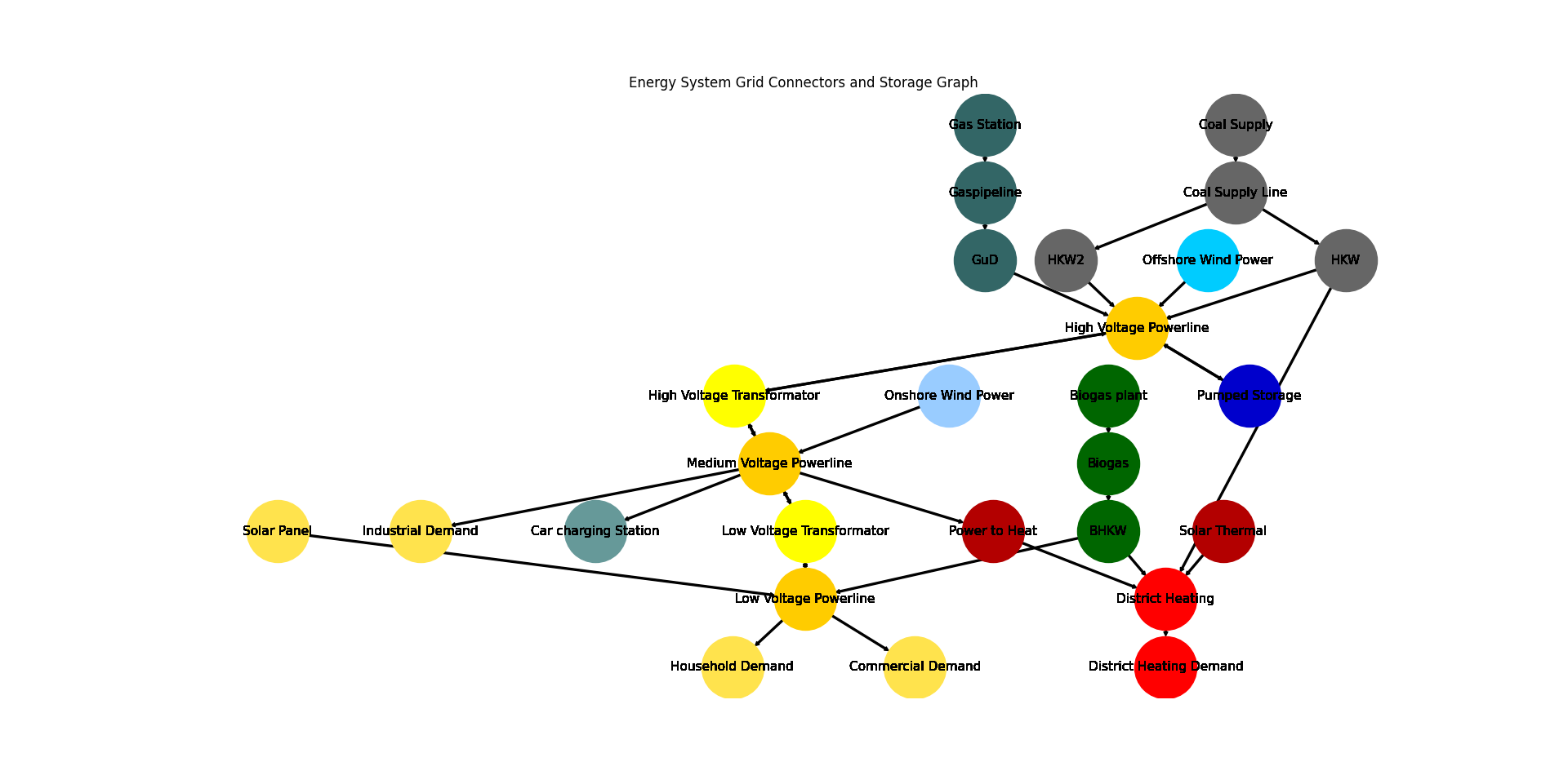
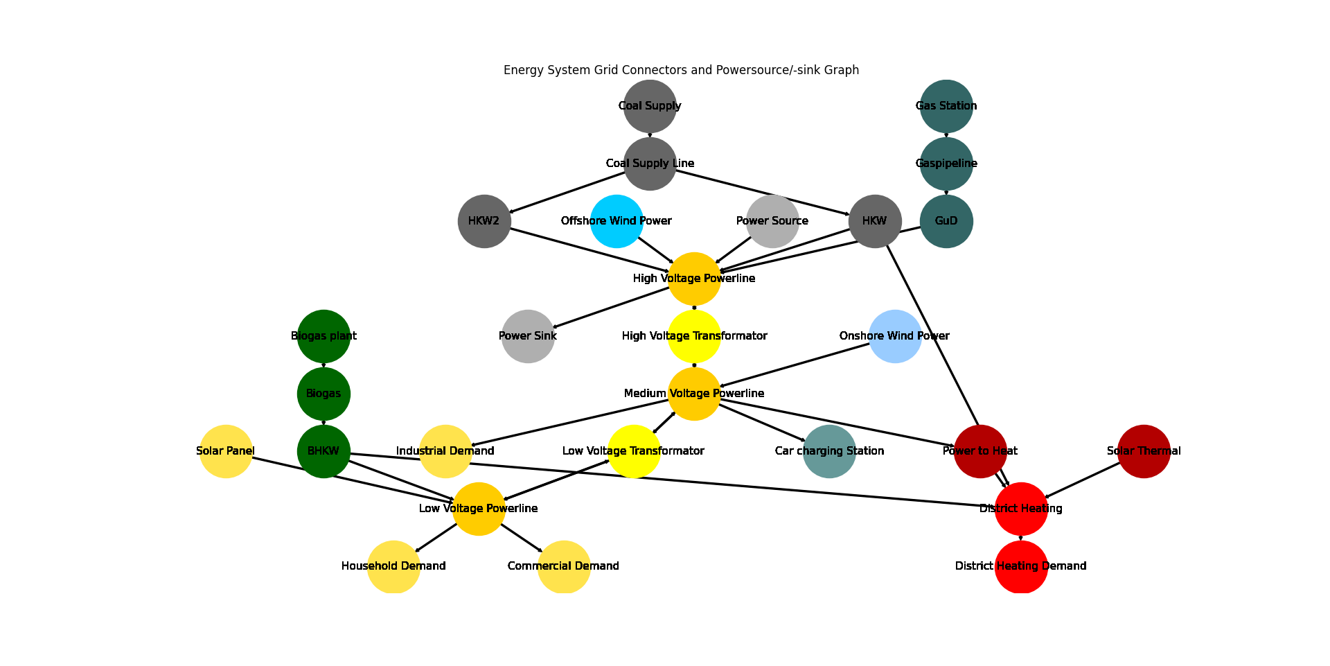
tessif.examples.data.tsf.py_hard.create_grid_cs_es(periods=24, transformer_efficiency=0.99, directory=None, filename=None)

Create a model of a generic grid style energy system using tessif's model.

Parameters:

• periods (int, default=24) – Number of time steps of the evaluated timeframe (one time step is one hour)

• transformer_efficiency (int, default=0.99) – Efficiency of the grid transformers (must be a value between 0 and 1)

• directory (str, default=None) –

  String representing of the path the created energy system is dumped to. Passed to dump() .

  Will be joined with filename.

  If set to None (default) tessif.frused.paths.write_dir/tsf will be the chosen directory.

• filename (str, default=None) –

  dump() the energy system using this name.

  If set to None (default) filename will be grid_es_CS.tsf.

Returns:

es – Tessif energy system.

Return type:

tessif.model.energy_system.AbstractEnergySystem

References

Minimum Working Example - For a step by step explanation on how to create a Tessif energy system.

Generic Grid Example (Brief) - For simulating and comparing this energy system using different supported models.

Grid Focused Model Scenario Combinations, - For a comprehensive example on a reference energy system to analyze and compare commitment optimization respecting among models.

Examples

Use create_grid_cs_es() to quickly access a tessif energy system to use for doctesting, or trying out this framework’s utilities.

>>> import tessif.examples.data.tsf.py_hard as tsf_py
>>> es = tsf_py.create_grid_cs_es()

>>> for node in es.nodes:
...     print(node.uid)
Gaspipeline
Low Voltage Powerline
District Heating
Medium Voltage Powerline
High Voltage Powerline
Coal Supply Line
Biogas
Solar Panel
Gas Station
Onshore Wind Power
Offshore Wind Power
Coal Supply
Solar Thermal
Biogas plant
Household Demand
Commercial Demand
District Heating Demand
Industrial Demand
Car charging Station
BHKW
Power to Heat
GuD
HKW
HKW2
Pumped Storage
Low Voltage Transformator
High Voltage Transformator

Visualize the energy system for better understanding what the output means:

>>> import matplotlib.pyplot as plt
>>> import tessif.visualize.nxgrph as nxv
>>> grph = es.to_nxgrph()
>>> drawing_data = nxv.draw_graph(
...     grph,
...     node_color={
...         'Coal Supply': '#666666',
...         'Coal Supply Line': '#666666',
...         'HKW': '#666666',
...         'HKW2': '#666666',
...         'Solar Thermal': '#b30000',
...         'Heat Storage': '#cc0033',
...         'District Heating': 'Red',
...         'District Heating Demand': 'Red',
...         'Power to Heat': '#b30000',
...         'Biogas plant': '#006600',
...         'Biogas': '#006600',
...         'BHKW': '#006600',
...         'Onshore Wind Power': '#99ccff',
...         'Offshore Wind Power': '#00ccff',
...         'Gas Station': '#336666',
...         'Gaspipeline': '#336666',
...         'GuD': '#336666',
...         'Solar Panel': '#ffe34d',
...         'Commercial Demand': '#ffe34d',
...         'Household Demand': '#ffe34d',
...         'Industrial Demand': '#ffe34d',
...         'Car charging Station': '#669999',
...         'Low Voltage Powerline': '#ffcc00',
...         'Medium Voltage Powerline': '#ffcc00',
...         'High Voltage Powerline': '#ffcc00',
...         'High Voltage Transformator': 'yellow',
...         'Low Voltage Transformator': 'yellow',
...         'Pumped Storage': '#0000cc',
...     },
...     title='Energy System Grid Connectors and Storage Graph',
... )
>>> # plt.show()  # commented out for simpler doctesting

tessif.examples.data.tsf.py_hard.create_grid_cp_es(periods=24, transformer_efficiency=0.99, directory=None, filename=None)

Create a model of a generic grid style energy system using tessif's model.

Parameters:

• periods (int, default=24) – Number of time steps of the evaluated timeframe (one time step is one hour)

• transformer_efficiency (int, default=0.99) – Efficiency of the grid transformers (must be a value between 0 and 1)

• directory (str, default=None) –

  String representing of the path the created energy system is dumped to. Passed to dump() .

  Will be joined with filename.

  If set to None (default) tessif.frused.paths.write_dir/tsf will be the chosen directory.

• filename (str, default=None) –

  dump() the energy system using this name.

  If set to None (default) filename will be grid_es_CP.tsf.

Returns:

es – Tessif energy system.

Return type:

tessif.model.energy_system.AbstractEnergySystem

References

Minimum Working Example - For a step by step explanation on how to create a Tessif energy system.

Generic Grid Example (Brief) - For simulating and comparing this energy system using different supported models.

Grid Focused Model Scenario Combinations, - For a comprehensive example on a reference energy system to analyze and compare commitment optimization respecting among models.

Examples

Use create_grid_cp_es() to quickly access a tessif energy system to use for doctesting, or trying out this framework’s utilities.

>>> import tessif.examples.data.tsf.py_hard as tsf_py
>>> es = tsf_py.create_grid_cp_es()

>>> for node in es.nodes:
...     print(node.uid)
Gaspipeline
Low Voltage Powerline
District Heating
Medium Voltage Powerline
High Voltage Powerline
Coal Supply Line
Biogas
Solar Panel
Gas Station
Onshore Wind Power
Offshore Wind Power
Coal Supply
Solar Thermal
Biogas plant
Power Source
Household Demand
Commercial Demand
District Heating Demand
Industrial Demand
Car charging Station
Power Sink
BHKW
Power to Heat
GuD
HKW
HKW2
Low Voltage Transformator
High Voltage Transformator

Visualize the energy system for better understanding what the output means:

>>> import matplotlib.pyplot as plt
>>> import tessif.visualize.nxgrph as nxv
>>> grph = es.to_nxgrph()
>>> drawing_data = nxv.draw_graph(
...     grph,
...     node_color={
...         'Coal Supply': '#666666',
...         'Coal Supply Line': '#666666',
...         'HKW': '#666666',
...         'HKW2': '#666666',
...         'Solar Thermal': '#b30000',
...         'Heat Storage': '#cc0033',
...         'District Heating': 'Red',
...         'District Heating Demand': 'Red',
...         'Power to Heat': '#b30000',
...         'Biogas plant': '#006600',
...         'Biogas': '#006600',
...         'BHKW': '#006600',
...         'Onshore Wind Power': '#99ccff',
...         'Offshore Wind Power': '#00ccff',
...         'Gas Station': '#336666',
...         'Gaspipeline': '#336666',
...         'GuD': '#336666',
...         'Solar Panel': '#ffe34d',
...         'Commercial Demand': '#ffe34d',
...         'Household Demand': '#ffe34d',
...         'Industrial Demand': '#ffe34d',
...         'Car charging Station': '#669999',
...         'Low Voltage Powerline': '#ffcc00',
...         'Medium Voltage Powerline': '#ffcc00',
...         'High Voltage Powerline': '#ffcc00',
...         'High Voltage Transformator': 'yellow',
...         'Low Voltage Transformator': 'yellow',
...     },
...     title='Energy System Grid Connectors and Powersource/-sink Graph',
... )
>>> # plt.show()  # commented out for simpler doctesting

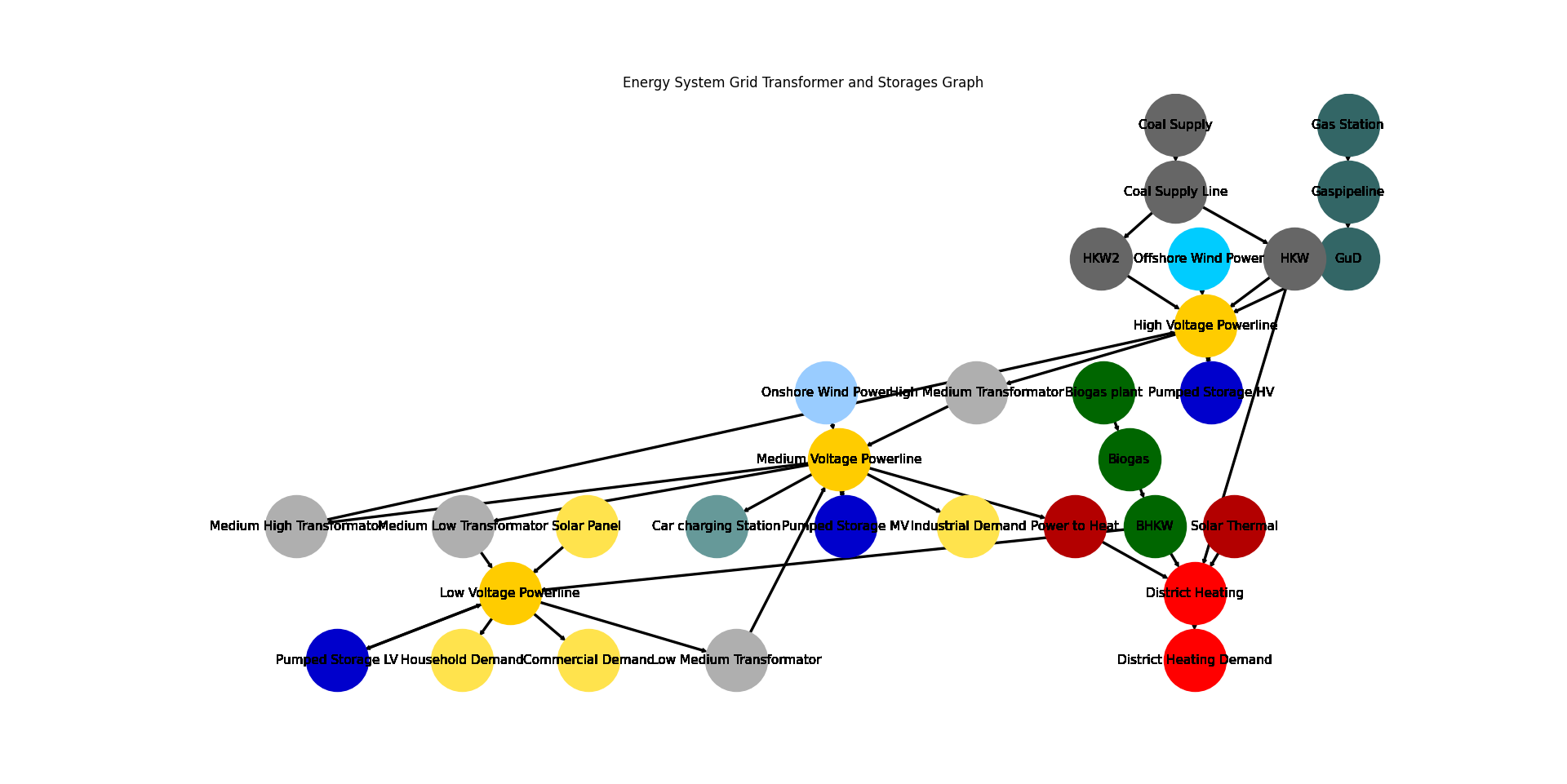
tessif.examples.data.tsf.py_hard.create_grid_ts_es(periods=24, transformer_efficiency=0.99, gridcapacity=60000, directory=None, filename=None)

Create a model of a generic grid style energy system using tessif's model.

Parameters:

• periods (int, default=24) – Number of time steps of the evaluated timeframe (one time step is one hour)

• transformer_efficiency (int, default=0.99) – Efficiency of the grid transformers (must be a value between 0 and 1)

• gridcapacity (int, default=60000) – Transmission capacity of the transformers of the gridstructure (at 0 the parts of the grid are not connected)

• directory (str, default=None) –

  String representing of the path the created energy system is dumped to. Passed to dump() .

  Will be joined with filename.

  If set to None (default) tessif.frused.paths.write_dir/tsf will be the chosen directory.

• filename (str, default=None) –

  dump() the energy system using this name.

  If set to None (default) filename will be grid_es_TS.tsf.

Returns:

es – Tessif energy system.

Return type:

tessif.model.energy_system.AbstractEnergySystem

References

Minimum Working Example - For a step by step explanation on how to create a Tessif energy system.

Generic Grid Example (Brief) - For simulating and comparing this energy system using different supported models.

Grid Focused Model Scenario Combinations, - For a comprehensive example on a reference energy system to analyze and compare commitment optimization respecting among models.

Examples

Use create_grid_ts_es() to quickly access a tessif energy system to use for doctesting, or trying out this framework’s utilities.

>>> import tessif.examples.data.tsf.py_hard as tsf_py
>>> es = tsf_py.create_grid_ts_es()

>>> for node in es.nodes:
...     print(node.uid)
Gaspipeline
Low Voltage Powerline
District Heating
Medium Voltage Powerline
High Voltage Powerline
Coal Supply Line
Biogas
Solar Panel
Gas Station
Onshore Wind Power
Offshore Wind Power
Coal Supply
Solar Thermal
Biogas plant
Household Demand
Commercial Demand
District Heating Demand
Industrial Demand
Car charging Station
BHKW
Power to Heat
GuD
HKW
High Medium Transformator
Low Medium Transformator
Medium Low Transformator
Medium High Transformator
HKW2
Pumped Storage LV
Pumped Storage MV
Pumped Storage HV

Visualize the energy system for better understanding what the output means:

>>> import matplotlib.pyplot as plt
>>> import tessif.visualize.nxgrph as nxv
>>> grph = es.to_nxgrph()
>>> drawing_data = nxv.draw_graph(
...     grph,
...     node_color={
...         'Coal Supply': '#666666',
...         'Coal Supply Line': '#666666',
...         'HKW': '#666666',
...         'HKW2': '#666666',
...         'Solar Thermal': '#b30000',
...         'Heat Storage': '#cc0033',
...         'District Heating': 'Red',
...         'District Heating Demand': 'Red',
...         'Power to Heat': '#b30000',
...         'Biogas plant': '#006600',
...         'Biogas': '#006600',
...         'BHKW': '#006600',
...         'Onshore Wind Power': '#99ccff',
...         'Offshore Wind Power': '#00ccff',
...         'Gas Station': '#336666',
...         'Gaspipeline': '#336666',
...         'GuD': '#336666',
...         'Solar Panel': '#ffe34d',
...         'Commercial Demand': '#ffe34d',
...         'Household Demand': '#ffe34d',
...         'Industrial Demand': '#ffe34d',
...         'Car charging Station': '#669999',
...         'Low Voltage Powerline': '#ffcc00',
...         'Medium Voltage Powerline': '#ffcc00',
...         'High Voltage Powerline': '#ffcc00',
...         'High Voltage Transformator': 'yellow',
...         'Low Voltage Transformator': 'yellow',
...         'Pumped Storage LV': '#0000cc',
...         'Pumped Storage MV': '#0000cc',
...         'Pumped Storage HV': '#0000cc',
...     },
...     title='Energy System Grid Transformer and Storages Graph',
... )
>>> # plt.show()  # commented out for simpler doctesting

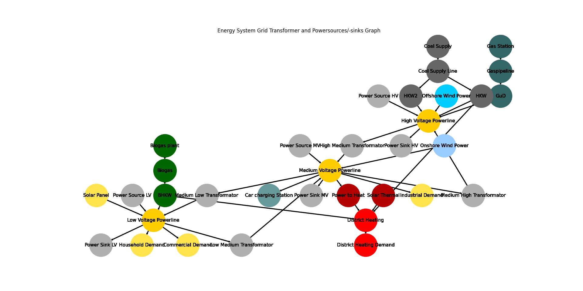
tessif.examples.data.tsf.py_hard.create_grid_tp_es(periods=24, transformer_efficiency=0.99, gridcapacity=60000, directory=None, filename=None)

Create a model of a generic grid style energy system using tessif's model.

Parameters:

• periods (int, default=24) – Number of time steps of the evaluated timeframe (one time step is one hour)

• transformer_efficiency (int, default=0.99) – Efficiency of the grid transformers (must be a value between 0 and 1)

• gridcapacity (int, default=60000) – Transmission capacity of the transformers of the gridstructure (at 0 the parts of the grid are not connected)

• directory (str, default=None) –

  String representing of the path the created energy system is dumped to. Passed to dump() .

  Will be joined with filename.

  If set to None (default) tessif.frused.paths.write_dir/tsf will be the chosen directory.

• filename (str, default=None) –

  dump() the energy system using this name.

  If set to None (default) filename will be grid_es_TP.tsf.

Returns:

es – Tessif energy system.

Return type:

tessif.model.energy_system.AbstractEnergySystem

References

Minimum Working Example - For a step by step explanation on how to create a Tessif energy system.

Generic Grid Example (Brief) - For simulating and comparing this energy system using different supported models.

Grid Focused Model Scenario Combinations, - For a comprehensive example on a reference energy system to analyze and compare commitment optimization respecting among models.

Examples

Use create_grid_tp_es() to quickly access a tessif energy system to use for doctesting, or trying out this framework’s utilities.

>>> import tessif.examples.data.tsf.py_hard as tsf_py
>>> es = tsf_py.create_grid_tp_es()

>>> for node in es.nodes:
...     print(node.uid)
Gaspipeline
Low Voltage Powerline
District Heating
Medium Voltage Powerline
High Voltage Powerline
Coal Supply Line
Biogas
Solar Panel
Offshore Wind Power
Onshore Wind Power
Gas Station
Coal Supply
Solar Thermal
Biogas plant
Power Source LV
Power Source MV
Power Source HV
Household Demand
Commercial Demand
District Heating Demand
Industrial Demand
Car charging Station
Power Sink LV
Power Sink MV
Power Sink HV
BHKW
Power to Heat
GuD
HKW
High Medium Transformator
Low Medium Transformator
Medium Low Transformator
Medium High Transformator
HKW2

Visualize the energy system for better understanding what the output means:

>>> import matplotlib.pyplot as plt
>>> import tessif.visualize.nxgrph as nxv
>>> grph = es.to_nxgrph()
>>> drawing_data = nxv.draw_graph(
...     grph,
...     node_color={
...         'Coal Supply': '#666666',
...         'Coal Supply Line': '#666666',
...         'HKW': '#666666',
...         'HKW2': '#666666',
...         'Solar Thermal': '#b30000',
...         'Heat Storage': '#cc0033',
...         'District Heating': 'Red',
...         'District Heating Demand': 'Red',
...         'Power to Heat': '#b30000',
...         'Biogas plant': '#006600',
...         'Biogas': '#006600',
...         'BHKW': '#006600',
...         'Onshore Wind Power': '#99ccff',
...         'Offshore Wind Power': '#00ccff',
...         'Gas Station': '#336666',
...         'Gaspipeline': '#336666',
...         'GuD': '#336666',
...         'Solar Panel': '#ffe34d',
...         'Commercial Demand': '#ffe34d',
...         'Household Demand': '#ffe34d',
...         'Industrial Demand': '#ffe34d',
...         'Car charging Station': '#669999',
...         'Low Voltage Powerline': '#ffcc00',
...         'Medium Voltage Powerline': '#ffcc00',
...         'High Voltage Powerline': '#ffcc00',
...         'High Voltage Transformator': 'yellow',
...         'Low Voltage Transformator': 'yellow',
...     },
...     title='Energy System Grid Transformer and Powersources/-sinks Graph',
... )
>>> # plt.show()  # commented out for simpler doctesting

tessif.examples.data.tsf.py_hard.create_transcne_es(periods=24, transformer_efficiency=0.93, gridcapacity=60000, expansion=False)

Create the TransCnE system model scenarios combinations.

As found in TransC/E – Transforer-Grid-Commitment/Expansion

Parameters:

• periods (int, default=24) – Number of time steps of the evaluated timeframe (one time step is one hour)

• transformer_efficiency (int, default=0.99) – Efficiency of the grid transformers (must be a value between 0 and 1)

• gridcapacity (int, default=60000) – Transmission capacity of the transformers of the grid structure (at 0 the parts of the grid are not connected)

• expansion (bool, default=False) – If True gridcapacity is subject to expansion.

Note

Changes compared to Hanke Project Thesis:

1. Rename "Power Source [Voltage]" to "Deficit Source [Voltage]"

2. Rename "Power Sinks [Voltage]" to "Excess Sinks [Voltage]"

3. Rename "[High/Mid/Low] Voltage Powerline" to "[High/Mid/Low] Voltage Grid"

4. Rename "[Voltage to Voltage] Transformator" to "[Voltage to Voltage] Transfer"

5. Change gridcapacity to reference the maximum outflow.

6. expansion capabilities are added to allow gridcapacity to be expanded

7. Default transformer_efficiency is decreased to 0.93 to discourage energy circulation between to grid busses to dissipate surplus amounts.

8. Outflow costs of 10 cost units per power unit are added to all Transfer components, to further discourage energy circulation between to grid busses to dissipate surplus amounts and to encourage local production and consumption.

Returns:

es – Tessif energy system.

Return type:

tessif.model.energy_system.AbstractEnergySystem

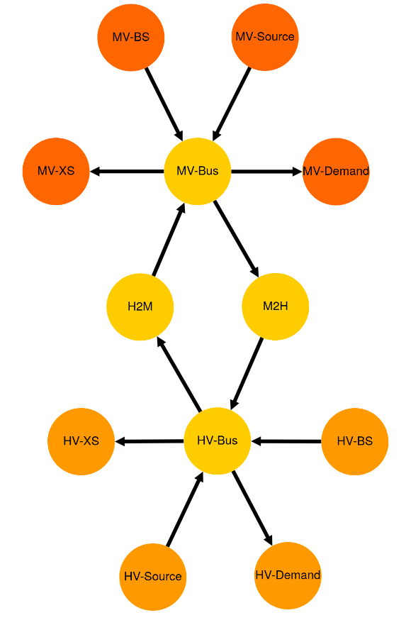
tessif.examples.data.tsf.py_hard.create_simple_transformer_grid_es(expansion=False)

Create a simplified grid energy system for testing.

Emulates common grid (congestion) behaviours, during its 6 timesteps:

1. Everything provided by HV-Source

2. Too much provided by HV-Source; H2M grid congests and MV-BS and MV-XS need to compensate

3. Too little provided, so MV-BS needs to provide

4. Everything provided by MV-Source

5. Too much provided by MV-Source, M2H grid congests and HV-BS and HV-XS need to compensate

6. Too little provided, so MV-BS needs to provide

Parameters:

expansion (bool) –

Boolean indicating whether to use the “expansion” model-scenario-combination. If True, the High -> Medium Voltage connection can be expanded at the cost of X per capacity, whereas the Medium -> High voltage connection can be expanded at the cost of 100 per capacity unit.

Leading to the first beeing expanded, so no redispatch has to be done from high to medium. The latter however will be not expanded, since redispatching from medium to high is more cost-efficient in this case.

The above behaviours subsequently change to:

1. Everything provided by HV-Source

2. Too much provided by HV-Source; It’s enough to also satisfy the MV-Demand, since the high to medium connection gets expanded. The HV-XS takes the excess indicating the amount of surpluss that would get capped in a real world application.

3. Too little provided, so MV-BS needs to provide

4. Everything provided by MV-Source

5. Too much provided by MV-Source, M2H grid congests and HV-BS and MV-XS need to compensate

6. Too little provided, so MV-BS needs to provide

Returns:

Tessif energy system model (scenario comibnation) emulating common grid analysis topics.

Return type:

tessif.model.energy_system.AbstractEnergySystem

Example

1. Create the Model-Scenario-Combination (msc):

>>> msc = create_simple_transformer_grid_es()

2. Optimize using oemof and see the results:

   import tessif.transform.es2es.omf as tsf2omf  # nopep8
   import tessif.simulate as optimize  # nopep8
   import tessif.transform.es2mapping.omf as post_process_omf  # nopep8
   
   omf_es = tsf2omf.transform(msc)
   opt_omf_es = optimize.omf_from_es(omf_es)
   all_res = post_process_omf.AllResultier(opt_omf_es)
   
   print(all_res.node_load['MV-Bus'])
   print(all_res.node_load['HV-Bus'])
   

3. Visualize the tessif energy system as generic graph:

>>> import tessif.visualize.dcgrph as dcv  # nopep8
>>> app = dcv.draw_generic_graph(
...     energy_system=msc,
...     color_group={
...         'HV-Demand': '#ff9900',
...         'HV-BS': '#ff9900',
...         'HV-XS': '#ff9900',
...         'HV-Source': '#ff9900',
...         'H2M': '#ffcc00',
...         'M2H': '#ffcc00',
...         'MV-Bus': '#ffcc00',
...         'HV-Bus': '#ffcc00',
...         'MV-Demand': '#ff6600',
...         'MV-Source': '#ff6600',
...         'MV-BS': '#ff6600',
...         'MV-XS': '#ff6600',
...     },
... )

>>> # commented out for doctesting. Uncomment to serve interactive drawing
>>> # to http://127.0.0.1:8050/
>>> # app.run_server(debug=False)

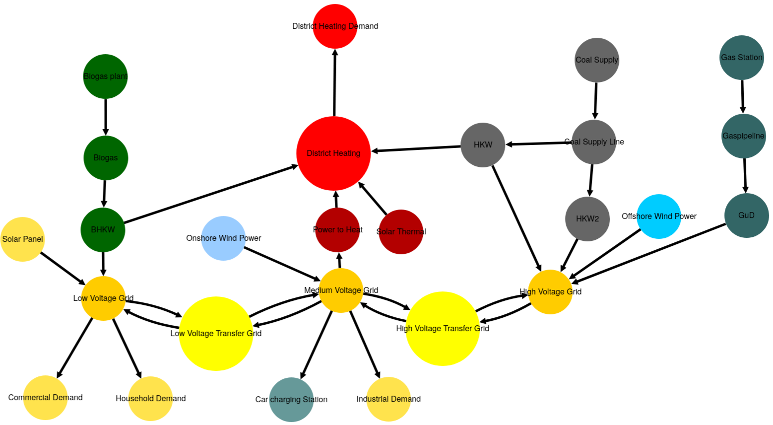
tessif.examples.data.tsf.py_hard.create_losslc_es(periods=24)

Create the TransCnE system model scenarios combinations.

Parameters:

periods (int, default=24) – Number of time steps of the evaluated timeframe (one time step is one hour)

Note

Changes compared to Hanke Project Thesis:

1. Rename "[High/Mid/Low] Voltage Powerline" to "[High/Mid/Low] Voltage Grid"

2. Rename "[High/Low] Voltage Transformator" to "[High/Low] Voltage Transfer Grid"

Returns:

es – Tessif energy system.

Return type:

tessif.model.energy_system.AbstractEnergySystem

Examples

Visualize the energy system:

>>> import tessif.visualize.dcgrph as dcv  # nopep8
>>> app = dcv.draw_generic_graph(
...     energy_system=create_losslc_es(),
...     color_group={
...         'Coal Supply': '#666666',
...         'Coal Supply Line': '#666666',
...         'HKW': '#666666',
...         'HKW2': '#666666',
...         'Solar Thermal': '#b30000',
...         'Heat Storage': '#cc0033',
...         'District Heating': 'Red',
...         'District Heating Demand': 'Red',
...         'Power to Heat': '#b30000',
...         'Biogas plant': '#006600',
...         'Biogas': '#006600',
...         'BHKW': '#006600',
...         'Onshore Wind Power': '#99ccff',
...         'Offshore Wind Power': '#00ccff',
...         'Gas Station': '#336666',
...         'Gaspipeline': '#336666',
...         'GuD': '#336666',
...         'Solar Panel': '#ffe34d',
...         'Commercial Demand': '#ffe34d',
...         'Household Demand': '#ffe34d',
...         'Industrial Demand': '#ffe34d',
...         'Car charging Station': '#669999',
...         'Low Voltage Grid': '#ffcc00',
...         'Medium Voltage Grid': '#ffcc00',
...         'High Voltage Grid': '#ffcc00',
...         'High Voltage Transfer Grid': 'yellow',
...         'Low Voltage Transfer Grid': 'yellow',
...     },
...     node_size={
...         'High Voltage Transfer Grid': 150,
...         'Low Voltage Transfer Grid': 150,
...         'District Heating': 150,
...     },
... )

>>> # commented out for doctesting. Uncomment to serve interactive drawing
>>> # to http://127.0.0.1:8050/
>>> # app.run_server(debug=False)

py_hard._create_minimal_es_unit(timeframe=None, seed=None)

Create a minimal self simular energy system unit.

Is used by create_self_similar_energy_system().

The self similar energy system unit consists of:

• 3 Source objects:

  • One having a randomized output, emulating renewable sources. With an installed power between 10 and 200 units.

  • One slack source providing energy to balance the system if needed. (This could be interpreted as an import node, for meeting load demands)

  • One commodity source feeding the transformer

• 2 Sink objects:

  • One having a fixed input with a net demand between 50 and 100 units.

  • One slack sink taking energy in to balance the system if needed. (This could be interpreted as an export node, for handling excess loads.)

• 2 Bus objects:

  • One central bus connecting the storage and transformer, as well as the sinks and sources and up to 2 additional self similar energy system units.

  • An auxiliary bus connecting the transformer and the central bus

• 1 Transformer object:

  • Fully parameterized transformer emulating a coal power plant with an installed capacity between 50 and 100 units.

• 1 Storage object:

  • no constraints to in and outflow. Efficiency, losses, expansion investment etc. oriented at grid level batteries (e.g. tesla)

Parameters:

• n (int) – Number of the es unit. This ist needed to be able to give each component in the complete self similar es a unique name.

• timeframe (pandas.DatetimeIndex) –

  Datetime index representing the evaluated timeframe. Explicitly stating:

  • initial datatime (0th element of the pandas.DatetimeIndex)

  • number of time steps (length of pandas.DatetimeIndex)

  • temporal resolution (pandas.DatetimeIndex.freq)

  For example:

  idx = pd.DatetimeIndex(
      data=pd.date_range(
          '2016-01-01 00:00:00', periods=11, freq='H'))