Grid Focused Model Scenario Combinations
When comparing energy system simulation models it makes sense to establish a common test base on which they can actually be compared.
The Application/scenarios
example module aggregates explanatory details on how to use tessif’s
comparing utilities on a set of grid based bench
mark scenarios to obtain meaningful results.
Further more it illustrates how these utilities can be used in a scientific context.
Introduction
This section includes a basic grid-based energy system model as well as various variations of this model.
These scenarios do not attempt to imitate an existing energy supply system, but are oriented towards a possible future energy supply system for Germany. In particular, the structure of the energy system is reflected in the models.
These scenarios are modeled and optimized with Oemof and PyPSA using Tessif to allow comparison of Oemof and PyPSA.
Reference Energy Systems
The basic energy system model create_grid_kp_es consists
of three different voltage levels (high, medium and low voltage).
These individual networks are interconnected by power transformers
(connector component).
Various consumers (households, commercial consumers, industrial consumers and charging stations for electric vehicles),
renewable energy sources (solar and onshore/offshore wind energy) and conventional power plants
(coal-fired cogeneration plant, combined cycle power plant and biogas CHP) are connected to the voltage levels.
In addition, there is a sector coupling with the heat sector. The electricity can be converted into heat directly
via Power-to-Heat.
The base model is considered lossless and without limitation of the transmission power between the voltage levels.
Energy System Graph
>>> import matplotlib.pyplot as plt
>>> import tessif.visualize.nxgrph as nxv
>>> grph = es.to_nxgrph()
>>> drawing_data = nxv.draw_graph(
...     grph,
...     node_color={
...         'Coal Supply': '#666666',
...         'Coal Supply Line': '#666666',
...         'HKW': '#666666',
...         'HKW2': '#666666',
...         'Solar Thermal': '#b30000',
...         'Heat Storage': '#cc0033',
...         'District Heating': 'Red',
...         'District Heating Demand': 'Red',
...         'Power to Heat': '#b30000',
...         'Biogas plant': '#006600',
...         'Biogas': '#006600',
...         'BHKW': '#006600',
...         'Onshore Wind Power': '#99ccff',
...         'Offshore Wind Power': '#00ccff',
...         'Gas Station': '#336666',
...         'Gaspipeline': '#336666',
...         'GuD': '#336666',
...         'Solar Panel': '#ffe34d',
...         'Commercial Demand': '#ffe34d',
...         'Household Demand': '#ffe34d',
...         'Industrial Demand': '#ffe34d',
...         'Car charging Station': '#669999',
...         'Low Voltage Powerline': '#ffcc00',
...         'Medium Voltage Powerline': '#ffcc00',
...         'High Voltage Powerline': '#ffcc00',
...         'High Voltage Transformator': 'yellow',
...         'Low Voltage Transformator': 'yellow',
...     },
...     title='Energy System Grid "Kupferplatte" Graph',
... )
>>> # plt.show()  # commented out for simpler doctesting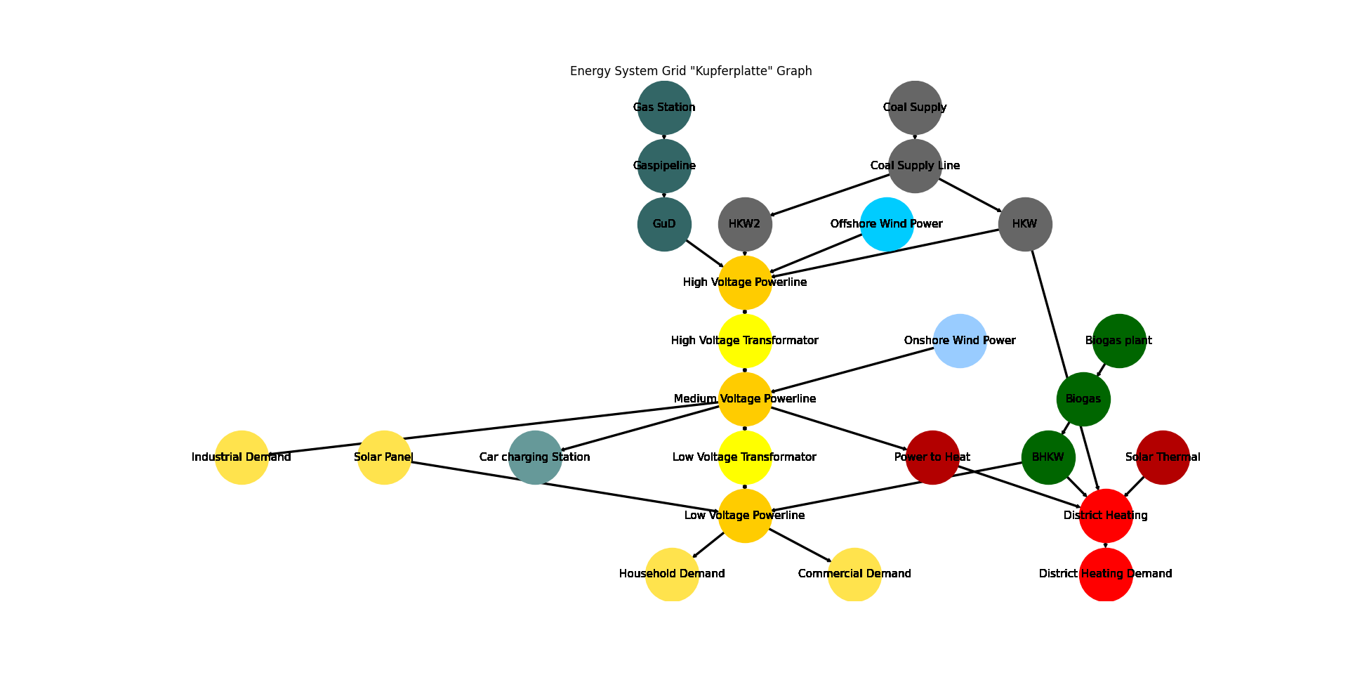
Model variations
There are different model variations to allow both transmission losses, but also grid limitation. Furthermore, the optimization capability of the energy system is improved by adding various components. A basic distinction can be made between models that are capable of limiting the transmission power between voltage levels and those that are not.
To enable network limitation, the voltage levels must be connected by two
transformer components each instead of connectors.
Models without grid limitation
The model create_grid_cs_es is able to represent
transmission losses of the grid transformer and also has an energy storage connected to the high-voltage level as a
further component.
The model create_grid_cp_es is also capable of representing
transmission losses. Instead of the storage unit, an unlimited power source/sink is integrated into the high-voltage
level.
These can be used to compensate for power surpluses and deficits.
Models with grid limitation
In addition to transmission losses, the
model create_grid_ts_es can also take into account a
limitation of the network. This model is also extended by an energy storage system.
However, a separate energy storage system is installed in each voltage level.
The model create_grid_tp_es can also represent the losses
as well as the grid limitation. This model is equipped with an unlimited power source/sink in each voltage level.
Model Results
In the following section, it is shown how to perform the optimization of the basic model using Oemof and PyPSA. Furthermore, it is shown how to evaluate the results with Tessif. As a result, the summed input and output powers of the components are given in GW. For the model variations, the optimization and evaluation can be performed in the same way. Therefore, only the results are shown.
Basic model (Kupferplattenmodell, create_grid_kp_es)
>>> import tessif.frused.configurations as configurations
>>> configurations.spellings_logging_level = 'debug'
>>> import pandas as pd
>>> # Import hardcoded Tessif energy system
>>> import tessif.examples.data.tsf.py_hard as tsf_py
>>> es = tsf_py.create_grid_kp_es()
>>> # Oemof optimization
>>> # Transform Tessif energy system into Oemof energy system
>>> from tessif.transform.es2es.omf import transform
>>> oemof_es = transform(es)
>>> # Optimize Oemof energy system
>>> import tessif.simulate as simulate
>>> optimized_oemof_es = simulate.omf_from_es(oemof_es)
>>> # Import the post processing utilities and conduct the post processing
>>> import tessif.transform.es2mapping.omf as oemof_results
>>> resultier_oemof = oemof_results.LoadResultier(optimized_oemof_es)
>>> resultier_oemof2 = oemof_results.IntegratedGlobalResultier(optimized_oemof_es)
>>> # PyPSA optimizartion
>>> # Transform Tessif energy system into PyPSA energy system
>>> from tessif.transform.es2es import ppsa as tsf2pypsa
>>> pypsa_es = tsf2pypsa.transform(es)
>>> # Optimize PyPSA energy system
>>> import tessif.simulate as simulate
>>> optimized_pypsa_es = simulate.ppsa_from_es(pypsa_es)
>>> # Import the post processing utilities and conduct the post processing
>>> from tessif.transform.es2mapping import ppsa as pypsa_results
>>> resultier_pypsa = pypsa_results.LoadResultier(optimized_pypsa_es)
>>> resultier_pypsa2 = pypsa_results.IntegratedGlobalResultier(optimized_pypsa_es)
>>> # Evaluation and output of results
>>> # Integrated Global Results
>>> IGR = pd.DataFrame([[resultier_oemof2.global_results['emissions (sim)'], resultier_pypsa2.global_results['emissions (sim)']],
...                    [resultier_oemof2.global_results['costs (sim)'], resultier_pypsa2.global_results['costs (sim)']]],
...                    columns=['Oemof', 'PyPSA'], index=['Emissions in t CO2', 'Costs in €'])
>>> print(IGR)
                          Oemof        PyPSA
Emissions in t CO2     443159.0     443159.0
Costs in €          202259102.0  202259102.0
>>> # Summed input and output powers
>>> result1 = pd.concat([resultier_oemof.node_load['Low Voltage Powerline'].sum()*-0.001,
...                      resultier_pypsa.node_load['Low Voltage Powerline'].sum()*-0.001],
...                      keys=['Oemof', 'PyPSA'], axis=1)
>>> result2 = pd.concat([resultier_oemof.node_load['Medium Voltage Powerline'].sum()*-0.001,
...                      resultier_pypsa.node_load['Medium Voltage Powerline'].sum()*-0.001],
...                      keys=['Oemof', 'PyPSA'], axis=1)
>>> result3 = pd.concat([resultier_oemof.node_load['High Voltage Powerline'].sum()*-0.001,
...                      resultier_pypsa.node_load['High Voltage Powerline'].sum()*-0.001],
...                      keys=['Oemof', 'PyPSA'], axis=1)
>>> result4 = pd.concat([resultier_oemof.node_load['District Heating'].sum()*-0.001,
...                      resultier_pypsa.node_load['District Heating'].sum()*-0.001],
...                      keys=['Oemof', 'PyPSA'], axis=1)
>>> result = pd.concat([result1, result2, result3, result4], keys=['Low Voltage Powerline', 'Medium Voltage Powerline',
...                                                                 'High Voltage Powerline', 'District Heating'])
>>> print(result)
                                                           Oemof        PyPSA
Low Voltage Powerline    BHKW                           8.774095     8.774096
                         Low Voltage Transformator    644.028627   644.028627
                         Solar Panel                  593.346832   593.346832
                         Commercial Demand           -582.459558  -582.459558
                         Household Demand            -552.564843  -552.564842
                         Low Voltage Transformator   -111.125154  -111.125154
Medium Voltage Powerline High Voltage Transformator   871.089257   871.089257
                         Low Voltage Transformator    111.125154   111.125154
                         Onshore Wind Power          1099.866419  1099.866419
                         Car charging Station         -37.026338   -37.026338
                         High Voltage Transformator    -0.000000    -0.000000
                         Industrial Demand          -1229.008356 -1229.008357
                         Low Voltage Transformator   -644.028627  -644.028627
                         Power to Heat               -172.017506  -172.017506
High Voltage Powerline   GuD                          121.996114   121.996114
                         HKW                          237.669821   237.669820
                         HKW2                         201.601795   201.601796
                         High Voltage Transformator    -0.000000    -0.000000
                         Offshore Wind Power          309.821525   309.821525
                         High Voltage Transformator  -871.089257  -871.089257
District Heating         BHKW                          13.825848    13.825848
                         HKW                          594.174551   594.174550
                         Power to Heat                172.017506   172.017506
                         Solar Thermal                 85.441944    85.441944
                         District Heating Demand     -865.459850  -865.459849
No differences in the optimization can be seen. It should be noted that Tessif determines the emissions for PyPSA in post processing via the energy flows, since the values of PyPSA cannot be tapped directly. Thus, different emissions may occur internally to the model.
Model without grid limitation and storage unit (create_grid_cs_es)
>>> print(IGR)
                          Oemof        PyPSA
Emissions in t CO2     460354.0     454697.0
Costs in €          200821160.0  199646851.0
>>> print(result)
                                                           Oemof        PyPSA
Low Voltage Powerline    BHKW                           2.909165     2.029346
                         Low Voltage Transformator    649.893559   650.773377
                         Solar Panel                  593.346832   593.346832
                         Commercial Demand           -582.459558  -582.459558
                         Household Demand            -552.564843  -552.564842
                         Low Voltage Transformator   -111.125154  -111.125154
Medium Voltage Powerline High Voltage Transformator   823.327705   819.948388
                         Low Voltage Transformator    110.013902   111.125154
                         Onshore Wind Power          1099.866419  1099.866419
                         Car charging Station         -37.026338   -37.026338
                         High Voltage Transformator    -0.000000    -0.000000
                         Industrial Demand          -1229.008356 -1229.008357
                         Low Voltage Transformator   -656.458141  -650.773377
                         Power to Heat               -110.715195  -114.131888
High Voltage Powerline   GuD                           78.789074    72.550369
                         HKW                          265.887430   265.075304
                         HKW2                         198.048698   193.560970
                         High Voltage Transformator    -0.000000    -0.000000
                         Offshore Wind Power          309.821525   309.821525
                         Pumped Storage                59.533591    59.980085
                         High Voltage Transformator  -831.644150  -819.948388
                         Pumped Storage               -80.436169   -81.039866
District Heating         BHKW                           4.584138     3.197758
                         HKW                          664.718572   662.688259
                         Power to Heat                110.715195   114.131888
                         Solar Thermal                 85.441944    85.441944
                         District Heating Demand     -865.459850  -865.459849
When comparing Oemof and PyPSA, it is noticeable that the PyPSA model is both cheaper and has lower emissions. This is due to the fact that PyPSA cannot represent transmission losses via connector components. The lower cost and higher emissions compared to the basic model are due to the impact of energy storage.
Model without grid limitation and power source/sink (create_grid_cp_es)
>>> print(IGR)
                          Oemof        PyPSA
Emissions in t CO2     448623.0     443159.0
Costs in €          203465454.0  202259102.0
>>> print(result)
                                                           Oemof        PyPSA
Low Voltage Powerline    BHKW                          10.422229     8.774096
                         Low Voltage Transformator    642.380495   644.028627
                         Solar Panel                  593.346832   593.346832
                         Commercial Demand           -582.459558  -582.459558
                         Household Demand            -552.564843  -552.564842
                         Low Voltage Transformator   -111.125154  -111.125154
Medium Voltage Powerline High Voltage Transformator   872.781594   871.089257
                         Low Voltage Transformator    110.013902   111.125154
                         Onshore Wind Power          1099.866419  1099.866419
                         Car charging Station         -37.026338   -37.026338
                         High Voltage Transformator    -0.000000    -0.000000
                         Industrial Demand          -1229.008356 -1229.008357
                         Low Voltage Transformator   -648.869188  -644.028627
                         Power to Heat               -167.758037  -172.017506
High Voltage Powerline   GuD                          126.908111   121.996114
                         HKW                          238.334786   237.669820
                         HKW2                         206.533148   201.601796
                         High Voltage Transformator    -0.000000    -0.000000
                         Offshore Wind Power          309.821525   309.821525
                         Power Source                  -0.000000    -0.000000
                         High Voltage Transformator  -881.597570  -871.089257
                         Power Sink                    -0.000000    -0.000000
District Heating         BHKW                          16.422906    13.825848
                         HKW                          595.836962   594.174550
                         Power to Heat                167.758037   172.017506
                         Solar Thermal                 85.441944    85.441944
                         District Heating Demand     -865.459850  -865.459849
Again, the differences in the modeling programs are due to the transmission efficiency of the connector. Since this is 100% for PyPSA, the optimization is identical to the base model.
Model with grid limitation and storage units (create_grid_ts_es)
>>> print(IGR)
                          Oemof        PyPSA
Emissions in t CO2     467832.0     467832.0
Costs in €          197240294.0  197240294.0
>>> print(result)
                                                          Oemof        PyPSA
Low Voltage Powerline    BHKW                          3.748359     3.748359
                         Medium Low Transformator    640.488831   640.104346
                         Pumped Storage LV            53.042050    51.950018
                         Solar Panel                 593.346832   593.346832
                         Commercial Demand          -582.459558  -582.459558
                         Household Demand           -552.564843  -552.564842
                         Low Medium Transformator    -83.942598   -83.942598
                         Pumped Storage LV           -71.659072   -70.182555
Medium Voltage Powerline High Medium Transformator   764.228788   762.902417
                         Low Medium Transformator     83.103172    83.103172
                         Onshore Wind Power         1099.866419  1099.866419
                         Pumped Storage MV            56.145835    53.481680
                         Car charging Station        -37.026338   -37.026338
                         Industrial Demand         -1229.008356 -1229.008357
                         Medium High Transformator    -0.000000    -0.000000
                         Medium Low Transformator   -646.958414  -646.570046
                         Power to Heat               -14.495461   -14.495461
                         Pumped Storage MV           -75.855645   -72.253488
High Voltage Powerline   GuD                          11.500603    11.500603
                         HKW                         303.846376   303.846376
                         HKW2                        164.165787   164.165787
                         Medium High Transformator    -0.000000    -0.000000
                         Offshore Wind Power         309.821525   309.821525
                         Pumped Storage HV            49.545702    53.350973
                         High Medium Transformator  -771.948270  -770.608502
                         Pumped Storage HV           -66.931723   -72.076762
District Heating         BHKW                          5.906505     5.906505
                         HKW                         759.615942   759.615940
                         Power to Heat                14.495461    14.495461
                         Solar Thermal                85.441944    85.441944
                         District Heating Demand    -865.459850  -865.459849
Identical results for Oemof and PyPSA. Both transmission efficiencies and network limitations can be achieved identically for both programs using Transformer components. Minor differences in the individual components are due to the effects of the energy storage.
Model with grid limitation and power sources/sinks (create_grid_tp_es)
>>> print(IGR)
                          Oemof        PyPSA
Emissions in t CO2     445925.0     445925.0
Costs in €          208059511.0  208059511.0
>>> print(result)
                                                          Oemof        PyPSA
Low Voltage Powerline    BHKW                         27.008983    27.008984
                         Medium Low Transformator    607.595379   607.595379
                         Power Source LV              18.198362    18.198362
                         Solar Panel                 593.346832   593.346832
                         Commercial Demand          -582.459558  -582.459558
                         Household Demand           -552.564843  -552.564842
                         Low Medium Transformator   -111.125154  -111.125154
                         Power Sink LV                -0.000000    -0.000000
Medium Voltage Powerline High Medium Transformator   837.645113   837.645112
                         Low Medium Transformator    110.013902   110.013902
                         Onshore Wind Power         1099.866419  1099.866419
                         Power Source MV              -0.000000    -0.000000
                         Car charging Station        -37.026338   -37.026338
                         Industrial Demand         -1229.008356 -1229.008357
                         Medium High Transformator    -0.000000    -0.000000
                         Medium Low Transformator   -613.732706  -613.732706
                         Power Sink MV                -0.000000    -0.000000
                         Power to Heat              -167.758037  -167.758037
High Voltage Powerline   GuD                          83.140093    83.140093
                         HKW                         227.880105   227.880103
                         HKW2                        225.264453   225.264453
                         Medium High Transformator    -0.000000    -0.000000
                         Offshore Wind Power         309.821525   309.821525
                         Power Source HV              -0.000000    -0.000000
                         High Medium Transformator  -846.106174  -846.106174
                         Power Sink HV                -0.000000    -0.000000
District Heating         BHKW                         42.559610    42.559611
                         HKW                         569.700257   569.700258
                         Power to Heat               167.758037   167.758037
                         Solar Thermal                85.441944    85.441944
                         District Heating Demand    -865.459850  -865.459849
Again, the optimization results of PyPSA and Oemof are identical. However, if the transmission of the grid is limited to 30,000 MW, PyPSA can no longer optimize the model. This is because PyPSA cannot make sinks variable and thus the excess power due to the grid limitation cannot be removed from the low voltage level. The following shows the command and the results of the grid limitation to 30,000 MW.
>>> # Import hardcoded Tessif energy system
>>> import tessif.examples.data.tsf.py_hard as tsf_py
>>> esys = tsf_py.create_grid_tp_es(24, 0.99, 30000, None, None)
>>> print(IGR)
                          Oemof
Emissions in t CO2     429778.0
Costs in €          253837370.0
>>> print(result)
                                                          Oemof
Low Voltage Powerline    BHKW                         97.417180
                         Medium Low Transformator    360.224135
                         Power Source LV             198.469179
                         Solar Panel                 593.346832
                         Commercial Demand          -582.459558
                         Household Demand           -552.564843
                         Low Medium Transformator   -110.645128
                         Power Sink LV                -3.787798
Medium Voltage Powerline High Medium Transformator   596.902146
                         Low Medium Transformator    109.538677
                         Onshore Wind Power         1099.866419
                         Power Source MV               6.151233
                         Car charging Station        -37.026338
                         Industrial Demand         -1229.008356
                         Medium High Transformator   -11.353142
                         Medium Low Transformator   -363.862763
                         Power Sink MV                -0.000000
                         Power to Heat              -171.207877
High Voltage Powerline   GuD                          -0.000000
                         HKW                         182.121669
                         HKW2                         99.748658
                         Medium High Transformator    11.239610
                         Offshore Wind Power         309.821525
                         Power Source HV              -0.000000
                         High Medium Transformator  -602.931459
                         Power Sink HV                -0.000000
District Heating         BHKW                        153.505860
                         HKW                         455.304168
                         Power to Heat               171.207877
                         Solar Thermal                85.441944
                         District Heating Demand    -865.459850
Conclusion
In summary, some differences exist between the optimizations using Oemof and PyPSA when considering grid-based energy systems. These are mostly due to limitations of the model components of Oemof or PyPSA. Whereas Oemof has no problems modeling grid-based energy systems. However, PyPSA is not able to specify transmission efficiencies for connectors. Furthermore, sinks cannot be made variable, so it is not possible to integrate an unlimited power sink into the model. Apart from the previously mentioned aspects, Oemof and PyPSA behave quite similarly in terms of optimization.
Used Utilities
grid_scenarios is a tessif
module aggregating the research results of a project thesis titled
Developing grid based scenarios for comparing free open source energy
supply system simulation software implemented in Python conducted by
YOUR_NAME.