Secondary Objectives

Tessif allows defining secondary objectives i.e. constraining global emissions to 0.

This is archieved by using the energy system's global_constraints parameter. Which allows to formulate any number of global constraints, like for example in the fully parameterized working example (fpwe).

Examples

Following sections demonstate the basic use of secondary objectives as well as some use case approaches for conveniently deploying different constraints and timeframes using the same externalized data set

Basic

Following example illustrates the basic use of global constraints for limiting an energy systems emissions.

Utilizing the example hub’s emission_objective() utility for conveniently accessing basic tessif energy system instance:
```
>>> from tessif.examples.data.tsf.py_hard import emission_objective
>>> tessif_es = emission_objective()
```

Display it’s global constraints:

>>> print(tessif_es.global_constraints)
{'emissions': 60}

Transform the tessif energy system into an oemof energy system for examplifying the perserverence of the global constraints:

>>> from tessif.transform.es2es.omf import transform
>>> oemof_es = transform(tessif_es)
>>> print(oemof_es.global_constraints)
{'emissions': 60}

>>> import tessif.examples.data.tsf.py_hard as tsf_py
>>> es = tsf_py.emission_objective()
>>> print(es.global_constraints['emissions'])
60

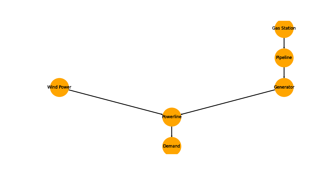
Visualize the energy system for better understanding what the output means:

>>> import matplotlib.pyplot as plt
>>> import tessif.visualize.nxgrph as nxv
>>> grph = es.to_nxgrph()
>>> drawing_data = nxv.draw_graph(
...     grph, node_color='orange')
>>> # plt.show()  # commented out for simpler doctesting

Optimize the energy system to see the constraint’s consequences:

>>> import tessif.simulate as simulate
>>> optimized_oemof_es = simulate.omf_from_es(oemof_es, solver='cbc')

>>> import tessif.transform.es2mapping.omf as oemof_results
>>> resultier = oemof_results.LoadResultier(optimized_oemof_es)

>>> # Generator costs/emissions are 2/1 unit respectively
>>> # Wind Power costs/emissions are 4/0 units respectively
>>> print(resultier.node_load['Powerline'])
Powerline            Gas Plant  Generator  Wind Power  Demand
1990-07-13 00:00:00       -5.0  -0.000000   -5.000000    10.0
1990-07-13 01:00:00       -5.0  -0.000000   -5.000000    10.0
1990-07-13 02:00:00       -5.0  -0.000000   -5.000000    10.0
1990-07-13 03:00:00       -5.0  -0.507246   -4.492754    10.0

Note how during the first 3 timesteps the more expensive wind power supply is used due to the emission constriants

Check global results using the dedicated resultier:

>>> ig_resultier = oemof_results.IntegratedGlobalResultier(optimized_oemof_es)
>>> import pprint
>>> pprint.pprint(ig_resultier.global_results)
{'capex (ppcd)': 0.0,
 'costs (sim)': 252.0,
 'emissions (sim)': 60.0,
 'opex (ppcd)': 252.0}

check the initial constraint:

>>> print(tessif_es.global_constraints)
{'emissions': 60}

Variable timeframes and constraints

Following example demonstrates how tessifs parsing capabilities simplify deploying different timeframes and sets of constraints to the same energy system. It also illustrates how expansion problems can be solved differently depending on the constraints stated.

Utilizing the example hub’s flat config files located in tessif/examples/data/tsf/cfg/flat/objectives for conveniently accessing basic tessif energy system data:

Create access to the path:

>>> import os
>>> from tessif.frused.paths import example_dir
>>> path = os.path.join(example_dir,
...     'data', 'tsf', 'cfg', 'flat', 'objectives')

silence the logger warnings:

>>> import tessif.frused.configurations as configurations
>>> configurations.spellings_logging_level = 'debug'

Create the actual energy system:

>>> import tessif.transform.mapping2es.tsf as ttsf
>>> import tessif.parse as parse
>>> tessif_es = ttsf.transform(
...     parse.flat_config_folder(
...        path,
...        timeframe='secondary',
...        global_constraints='primary'))

Note how the timeframe key 'secondary' correspond to the section header found in tessif/examples/data/tsf/cfg/flat/objectives.

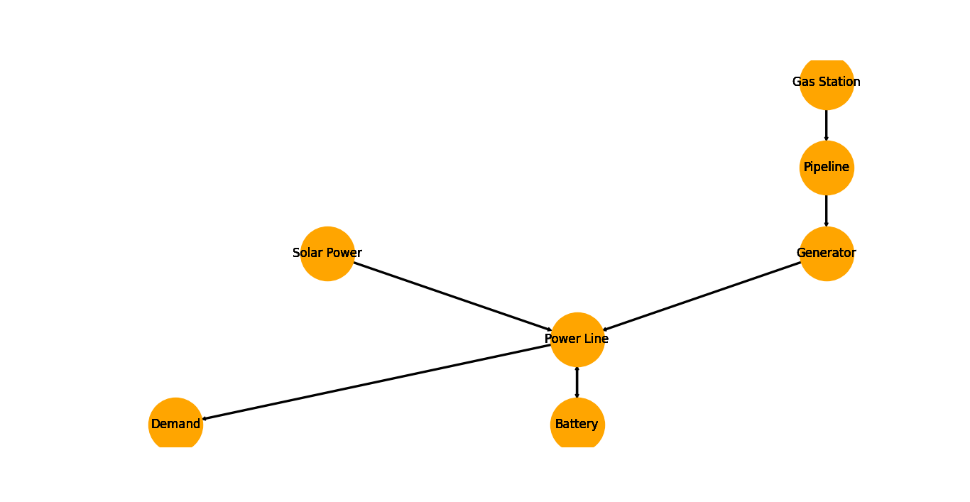
Visualize the energy system for better understanding what the output means:

>>> import matplotlib.pyplot as plt
>>> import tessif.visualize.nxgrph as nxv
>>> grph = tessif_es.to_nxgrph()
>>> drawing_data = nxv.draw_graph(
...     grph, node_color='orange')
>>> # plt.show()  # commented out for simpler doctesting

Display it’s global constraints:

>>> print(tessif_es.global_constraints)
{'name': 'default', 'emissions': inf, 'resources': inf}

Transform the tessif energy system into an oemof energy system for examplifying the perserverence of the global constraints:

>>> from tessif.transform.es2es.omf import transform
>>> oemof_es = transform(tessif_es)
>>> print(oemof_es.global_constraints)
{'name': 'default', 'emissions': inf, 'resources': inf}

Optimize the energy system to see the constraint’s consequences:

>>> import tessif.simulate as simulate
>>> optimized_oemof_es = simulate.omf_from_es(oemof_es, solver='cbc')

>>> import tessif.transform.es2mapping.omf as oemof_results
>>> resultier = oemof_results.LoadResultier(optimized_oemof_es)

>>> # Generator costs/emissions are 1/10 units respectively
>>> # Solar Power costs/emissions are 0/0 units respectively
>>> # but only 15 units are installed, expansion costs are 10 per unit
>>> print(resultier.node_load['Power Line'])
Power Line           Battery  Generator  Solar Power  Battery  Demand
2019-10-03 00:00:00     -0.0       -5.0        -15.0      0.0    20.0
2019-10-03 01:00:00     -0.0       -5.0        -15.0      0.0    20.0
2019-10-03 02:00:00     -0.0       -5.0        -15.0      0.0    20.0

Check global results using the dedicated resultier:

>>> ig_resultier = oemof_results.IntegratedGlobalResultier(optimized_oemof_es)
>>> import pprint
>>> pprint.pprint(ig_resultier.global_results)
{'capex (ppcd)': 0.0,
 'costs (sim)': 15.0,
 'emissions (sim)': 150.0,
 'opex (ppcd)': 15.0}

>>> # check the initial constraint:
>>> print(tessif_es.global_constraints)
{'name': 'default', 'emissions': inf, 'resources': inf}

Data file for reference:

# each source is denoted by its own section aka '[SECTION]'
[gas_station]
'name'='Gas Station'
'outputs'=('fuel',)
# Minimum number of arguments required
'latitude'=42
'longitude'=42
'region'='Here'
'sector'='Coupled'
'carrier'='Gas'
'node_type'='source'


[solar_panel]
'name'='Solar Power'
'outputs'=('electricity',)
# Minimum number of arguments required
'latitude'=42
'longitude'=42
'region'='Here'
'sector'='Power'
'carrier'='Electricity'
'node_type'='Renewable'

# solar panel undersized for soley providing energy, but expandable

'flow_rates'={'electricity': (15, 15)}
'flow_costs'={'electricity': 0}
'flow_emissions'={'electricity': 0}
# 'timeseries'={'electricity': (
#     [3, 5, 7, 10, 15, 12, 8, 2],
#     [3, 5, 7, 10, 15, 12, 8, 2])}
'expandable'={'electricity': True}
'expansion_costs'={'electricity': 10}
'expansion_limits'={'electricity': (15, '+inf')}

Change the parsed constraints:

>>> tessif_es = ttsf.transform(
...     parse.flat_config_folder(
...        path,
...        timeframe='secondary',
...        global_constraints='tertiary'))

>>> print(tessif_es.global_constraints)
{'name': '100% Reduction', 'emissions': 0.0, 'resources': inf}

Resimulate:

>>> oemof_es = transform(tessif_es)
>>> optimized_oemof_es = simulate.omf_from_es(oemof_es, solver='cbc')

Note how the emission constraint leads to the solar power beeing expanded (altough more expensive):

>>> resultier = oemof_results.LoadResultier(optimized_oemof_es)
>>> print(resultier.node_load['Power Line'])
Power Line           Battery  Generator  Solar Power  Battery  Demand
2019-10-03 00:00:00     -0.0       -0.0        -20.0      0.0    20.0
2019-10-03 01:00:00     -0.0       -0.0        -20.0      0.0    20.0
2019-10-03 02:00:00     -0.0       -0.0        -20.0      0.0    20.0

Recheck global results using the dedicated resultier (Note how the emissions are now 0 but the costs increased by 35 units and shifted from opex to capex):

>>> ig_resultier = oemof_results.IntegratedGlobalResultier(optimized_oemof_es)
>>> import pprint
>>> pprint.pprint(ig_resultier.global_results)
{'capex (ppcd)': 50.0,
 'costs (sim)': 50.0,
 'emissions (sim)': 0.0,
 'opex (ppcd)': 0.0}
# check the initial constraint: >>> print(tessif_es.global_constraints) {‘name’: ‘100% Reduction’, ‘emissions’: 0.0, ‘resources’: inf}