Identifcation of Differences
When comparing energy supply system modelling results between different softwares, load results for the exact same component may differ between those softwares,
The Application/timeseries_comparison
example module aggregates explanatory details on how to use tessif’s
comparing utilities for comparing load differences
between energy supply system modelling softwares modelling the same energy
supply system scenario combination.
Introduction
In order to work out differences between the results of different energy supply system modelling tools several steps are proposed, which are laid and discussed in the following sections.
Analyzed System-Model-Scenario-Combination
A system-model-scenario combination (from here on combination or msc) is
represented by the tessif ennergy system class which combines the model
itself (i.e its components, most of their parameters as well as their
interconnection) as well as the scenario formulation (i.e. timeframe,
commitment/expansion problem related parameters, as well as secodnary
constraints).
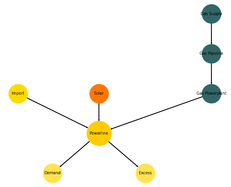
The used combination is deliberatey simple and called statistical example msc.
A generic graph representation of this combination can bee seen
in the figure below.
Generic Energy System Graph
Structrured Comparison
Initial code to do the comparison
>>> # change spellings_logging_level to debug to declutter output
>>> import tessif.frused.configurations as configurations
>>> configurations.spellings_logging_level = 'debug'
>>> # Import hardcoded tessif energy system using the example hub:
>>> from tessif.examples.application import timeseries_comparison
>>> # Choose the underlying energy system
>>> msc = timeseries_comparison.create_statistical_example_msc()
>>> # write it to disk, so the comparatier can read it out
>>> import os
>>> from tessif.frused.paths import write_dir
>>> #
>>> output_msg = msc.to_hdf5(
...     directory=os.path.join(write_dir, 'tsf'),
...     filename='statistical_example.hdf5',
... )
>>> # let the comparatier to the auto comparison:
>>> import tessif.analyze, tessif.parse
>>> #
>>> comparatier = tessif.analyze.Comparatier(
...     path=os.path.join(write_dir, 'tsf', 'statistical_example.hdf5'),
...     parser=tessif.parse.hdf5,
...     models=('oemof', 'pypsa', 'calliope'),
... )
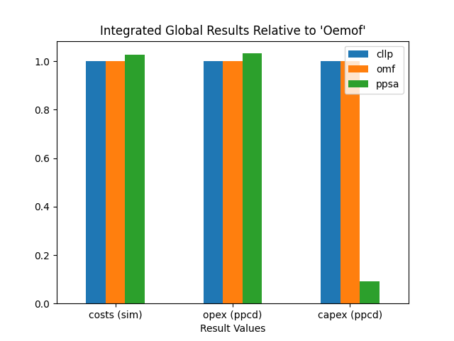
Integrated Global Results
The poposed first step in any software based comparison is to compare
the high priority or integrated global results:
>>> igr_results = comparatier.integrated_global_results.drop(
...     ['time (s)', 'memory (MB)'], axis='index')
>>> igr_results
                       cllp         omf        ppsa
emissions (sim)      9881.0      9881.0      6587.0
costs (sim)      14965855.0  14965855.0  15391316.0
opex (ppcd)      14900503.0  14900503.0  15385335.0
capex (ppcd)        65348.0     65348.0      5986.0
Visualize these results as bar plots seperated in costs and emissions:
>>> # make results relative to oemof
>>> igr_relative_results = igr_results.div(igr_results['omf'], axis='index')
>>> # configure the plot
>>> mpl_config = {
...     "title": "Integrated Global Results Relative to 'Oemof'",
...     "ylabel": "",
...     "xlabel": "Result Values",
...     "rot": 0,
... }
>>> # do the plotting
>>> from tessif.visualize import igr
>>> handle = igr.plot(
...     igr_df=igr_relative_results,
...     plt_config=mpl_config,
...     ptype="bar",
... )
>>> # handle["costs"].show()
>>> # handle["non_costs"].show()

This initial comparison reveals that oemof and calliope are likely
to come to the exact same result. Whereas pypsa seems to optimize the
msc differently.
Advanced Graphs
In cases general deviations are detected via the Integrated Global Results, comparing the attr:Advanced Graph <tessif.visualize.dcgrph.draw_advanced_graph> of each software is the next proposed step. These graphs as well as their respective code creation snippets are shown below.
Pypsa
Using the demand capacity and net energy flow as reference, since they are the same among all softwares, thus facilitating inter software comparison:
>>> import tessif.transform.es2mapping.ppsa as post_process_ppsa
>>> demand_capacity = post_process_ppsa.CapacityResultier(
...     optimized_es=comparatier.energy_systems["ppsa"]).node_installed_capacity[
...         "Demand"]
>>> demand_net_energy_flow = post_process_ppsa.FlowResultier(
...     optimized_es=comparatier.energy_systems["ppsa"]).edge_net_energy_flow[
...         ("Powerline", "Demand")]
>>> print(demand_capacity)
1389.632
>>> print(demand_net_energy_flow)
27905.41
Draw the advanced graph / advanced system visualization (AGS/AVS):
>>> import tessif.visualize.dcgrph as dcv  # nopep8
>>> app = dcv.draw_advanced_graph(
...     optimized_es=comparatier.energy_systems["ppsa"],
...     # layout='style',
...     # layout_nodeDimensionsIncludeLabels=True,
...     node_shape="circle",
...     node_color={
...         'Demand': '#ffe34d',
...         'Excess': '#ffe34d',
...         'Gas Supply': '#336666',
...         'Gas Pipeline': '#336666',
...         'Gas Powerplant': '#336666',
...         'Solar': '#FF7700',
...         'Powerline': '#ffcc00',
...         'Import': '#ffd900',
...     },
...     reference_node_width=demand_capacity,
...     reference_edge_width=demand_net_energy_flow,
... )
>>> # app.run_server()

Oemof
Using the demand capacity and net energy flow as reference, since they are the same among all softwares, thus facilitating inter software comparison:
>>> import tessif.transform.es2mapping.omf as post_process_omf
>>> demand_capacity = post_process_omf.CapacityResultier(
...     optimized_es=comparatier.energy_systems["omf"]).node_installed_capacity[
...         "Demand"]
>>> demand_net_energy_flow = post_process_omf.FlowResultier(
...     optimized_es=comparatier.energy_systems["omf"]).edge_net_energy_flow[
...         ("Powerline", "Demand")]
>>> print(demand_capacity)
1389.632
>>> print(demand_net_energy_flow)
27905.41
Draw the advanced graph / advanced system visualization (AGS/AVS):
>>> import tessif.visualize.dcgrph as dcv  # nopep8
>>> app = dcv.draw_advanced_graph(
...     optimized_es=comparatier.energy_systems["omf"],
...     # layout='style',
...     # layout_nodeDimensionsIncludeLabels=True,
...     node_shape="circle",
...     node_color={
...         'Demand': '#ffe34d',
...         'Excess': '#ffe34d',
...         'Gas Supply': '#336666',
...         'Gas Pipeline': '#336666',
...         'Gas Powerplant': '#336666',
...         'Solar': '#FF7700',
...         'Powerline': '#ffcc00',
...         'Import': '#ffd900',
...     },
...     reference_node_width=demand_capacity,
...     reference_edge_width=demand_net_energy_flow,
... )
>>> # app.run_server()

Identifying Key Differences
Next on the list of proposed steps for inter software comparisons is the identifcation of key differences. Wich breaks down into the tasks of identifying differing components, as well as timeframes on which they differ.
Identifying Differing Components
There are two different approaches to identify differing components, synergizing well with each other. The first is to visually detect discrepancies using the advanced graphs. The second is to use tessif’s statistical identification tools using a combination of correlation coefficients and normalize error values.
Visual Comparison on Advanced Graphs
Comparing the advanced graph visualizations, following deviations can be observed:
oemofsinstalledSolarcapacity is far greater than that ofpypsa
omeofuses theExcessssink far more thanpypsa
Leading to the conclusion, that the flows Solar -> Powerline and
Powerline -> Excess are probably the ones differing the most.
As well as the respective installed capacities of those two components.
Statistical Identification
In order to work out differences between the results of different energy supply system modelling softwares, several steps are necessary. First, a set of reference results has to be declared to which the obtained results are compared to. These reference results can be either one of the used software results or a fictional set of average/medium results. The latter is obtained by averageing the results of each each software for each component and timestep.
For automated identifcation tessif.identify.TimevaryingIdentificier is
used which clusters the interest of inter component flows by calculating a
correlation coefficient (usually the Pearson correlation Coefficient (PCC)) in
conjunction with a statistical error value (usually the
Normalized Mean Average Error) applied to a
Clustering Matrix.
In combination with respective threshold values for correlation coefficient
and error value, a level of interest is estimated in the sense of giving an
estimate of the value of futher investigations.
For the design case, the pearson correlation in conjunction with the normalized mean average error is used on following conditions and levels of interest:
PCC < 0.7 and N M AE > K = 10%; High interest / significantly different:
This case is of most interest to detect and diagnose differences between software models. A PCC of less then 0.7 implies differing dynamic component behaviour and a NMAE of greater equal 5% indicates that on top of the differing dynamics, the actually resulting differences are worth noting.
PCC < 0.7 and NMAE < K = 10%; Medium interest / boderline significantly different:
This case can be of interest to detect and diagnose differences between software models but is often just a side-effect. Like above, the P CC value less than 0.7 indicates differing diynamics. In this case however, these differences amount to only less than 5% in total.
PCC > 0.7 and NMAE > K = 10%; Medium interest / boderline significantly different:
Like the case above, this one describes also one of potential interest. A PCC value greater 0.7 indicates a somewhat synchronous dispatch pattern. In conjunction with a relatively high NMAE of greater 5% however, this means one component provides significantly more energy than the other. This is often just a side-effect of less emitive and/or cheaper components beeing more heavily constraint (be it direct or indirect) within some softwares.
PCC > 0.7 and N M AE < K = 10%; Least interesting / most likely of no interest:
This case marks the least interesting one. A PCC value greater 0.7 again implies a relatively synchronous dispatch pattern. In combination with a low NMAE this most often indicates, that the components behave very similar between the softwares compared.
During the identifcation process, the data is sorted and filtered, since particularities of certain tessif-software implementations may lead to discrepancies in actual components present inside the supply system model. This filtering ensures that only components are compared, that are actually present in all supply system models.
>>> from tessif.identify import TimevaryingIdentificier
>>> idf = TimevaryingIdentificier(
...     data=comparatier.comparative_results.all_loads,
...     error_value="nmae",
...     error_value_threshold=0.1,
...     correlation="pearson",
...     correlation_threshold=0.7,
...     # igr from above show oemof~calliope, hence reference=omf
...     reference="omf",
... )
>>> print(idf.clustered_interest)
                         cllp  omf    ppsa
Gas Powerplant Powerline  low  low    high
Import         Powerline  low  low     low
Powerline      Demand     low  low     low
               Excess     low  low    high
Solar          Powerline  low  low  medium
>>> print(idf.high)
                          ppsa
Gas Powerplant Powerline  high
Powerline      Excess     high
>>> print(idf.medium)
                   ppsa
Solar Powerline  medium
In addition to the prior identified flows Solar -> Powerline and
Powerline -> Excess the flow Gas Powerplant -> Powerline is also
recommended to be worth investigating.
Timevarying Result Data of Identified Components
To inspect the time varying result data (load results in this case) tessif offers two options:
>>> high_interest_flows = tuple(idf.high.index)
>>> print(high_interest_flows)
(('Gas Powerplant', 'Powerline'), ('Powerline', 'Excess'))
Use the
Identificier:>>> print(idf.high_interest_results[('Gas Powerplant', 'Powerline')]) cllp omf ppsa 2019-01-01 00:00:00 400.0 400.0 400.00000 2019-01-01 01:00:00 400.0 400.0 400.00000 2019-01-01 02:00:00 400.0 400.0 400.00000 2019-01-01 03:00:00 400.0 400.0 400.00000 2019-01-01 04:00:00 400.0 400.0 400.00000 2019-01-01 05:00:00 400.0 400.0 400.00000 2019-01-01 06:00:00 400.0 400.0 400.00000 2019-01-01 07:00:00 400.0 400.0 400.00000 2019-01-01 08:00:00 400.0 400.0 400.00000 2019-01-01 09:00:00 400.0 400.0 400.00000 2019-01-01 10:00:00 0.0 0.0 400.00000 2019-01-01 11:00:00 0.0 0.0 277.13932 2019-01-01 12:00:00 0.0 0.0 0.00000 2019-01-01 13:00:00 0.0 0.0 159.99420 2019-01-01 14:00:00 0.0 0.0 379.51340 2019-01-01 15:00:00 400.0 400.0 400.00000 2019-01-01 16:00:00 400.0 400.0 400.00000 2019-01-01 17:00:00 400.0 400.0 400.00000 2019-01-01 18:00:00 400.0 400.0 400.00000 2019-01-01 19:00:00 400.0 400.0 400.00000 2019-01-01 20:00:00 400.0 400.0 400.00000 2019-01-01 21:00:00 400.0 400.0 400.00000 2019-01-01 22:00:00 400.0 400.0 400.00000 2019-01-01 23:00:00 400.0 400.0 400.00000
Index the comparative results directly in case you are only interested in the results of certain softwares:
>>> print(comparatier.comparative_results.all_loads[
...     "ppsa"][('Gas Powerplant', 'Powerline')])
2019-01-01 00:00:00    400.00000
2019-01-01 01:00:00    400.00000
2019-01-01 02:00:00    400.00000
2019-01-01 03:00:00    400.00000
2019-01-01 04:00:00    400.00000
2019-01-01 05:00:00    400.00000
2019-01-01 06:00:00    400.00000
2019-01-01 07:00:00    400.00000
2019-01-01 08:00:00    400.00000
2019-01-01 09:00:00    400.00000
2019-01-01 10:00:00    400.00000
2019-01-01 11:00:00    277.13932
2019-01-01 12:00:00      0.00000
2019-01-01 13:00:00    159.99420
2019-01-01 14:00:00    379.51340
2019-01-01 15:00:00    400.00000
2019-01-01 16:00:00    400.00000
2019-01-01 17:00:00    400.00000
2019-01-01 18:00:00    400.00000
2019-01-01 19:00:00    400.00000
2019-01-01 20:00:00    400.00000
2019-01-01 21:00:00    400.00000
2019-01-01 22:00:00    400.00000
2019-01-01 23:00:00    400.00000
Name: (Gas Powerplant, Powerline), dtype: float64
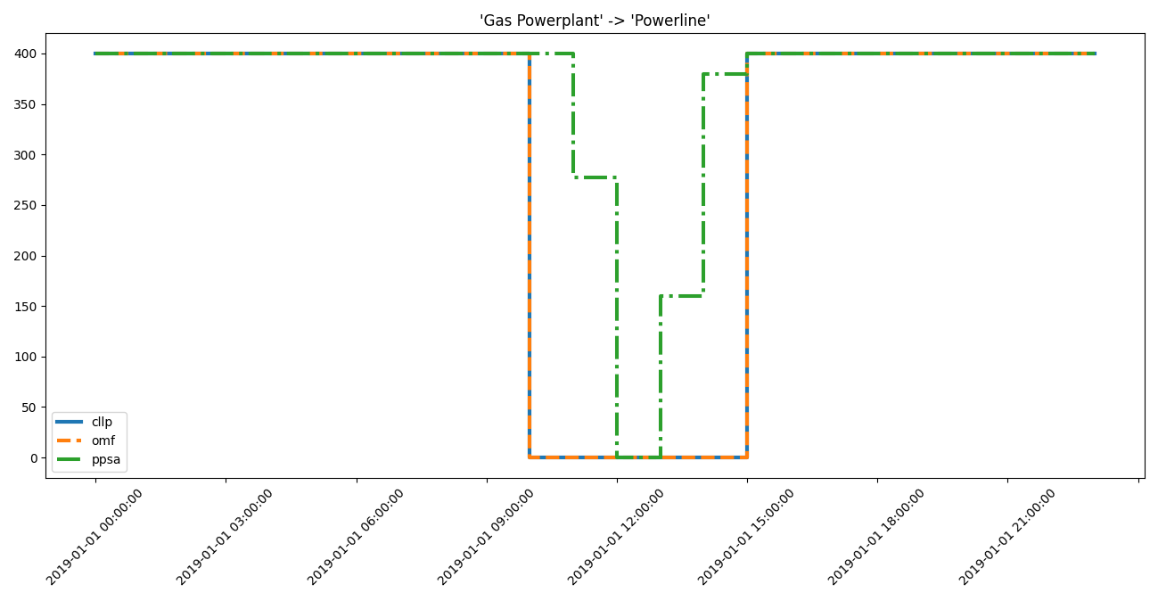
Visualizing Timevarying Result Data of Identified Components
Plotting the results for manual inspection:
>>> from tessif.visualize import component_loads
>>> axes = component_loads.step(
...     idf.high_interest_results[('Gas Powerplant', 'Powerline')])
>>> # axes.figure.show()  # commented out for doctesting
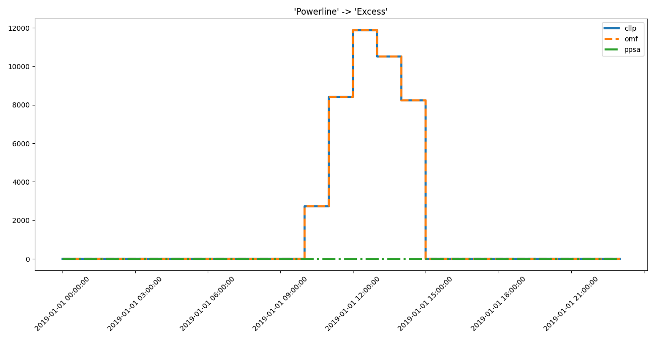
>>> axes = component_loads.step(
...     idf.high_interest_results[('Powerline', 'Excess')])
>>> # axes.figure.show()  # commented out for doctesting
>>> axes = component_loads.step(
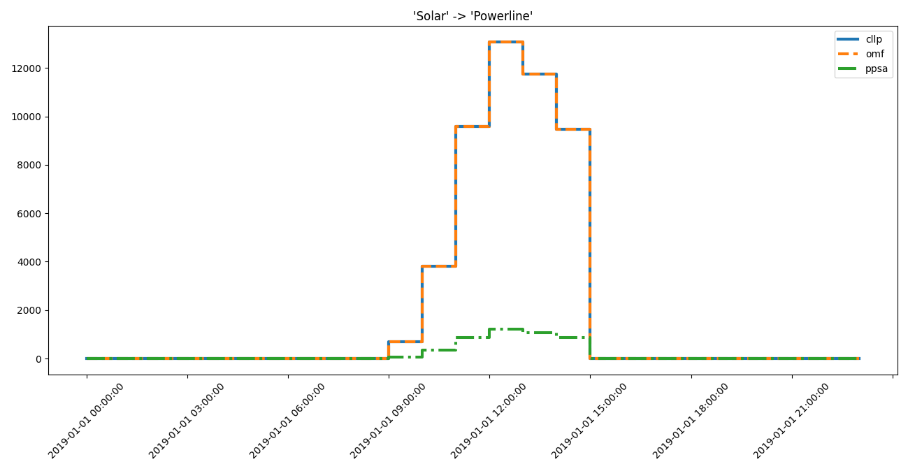
... idf.medium_interest_results[('Solar', 'Powerline')])
>>> # axes.figure.show() # commented out for doctesting
Identifying Differing Timeframes
On large scale data sets of many timesteps (e.g 8760 for a whole year of hourly
resolved results), the above method may not be the first, since there are
potentially a lot of data points where the results actually do not differ.
The Identificier however, provides
a convenient method to identify timeframes of significant difference:
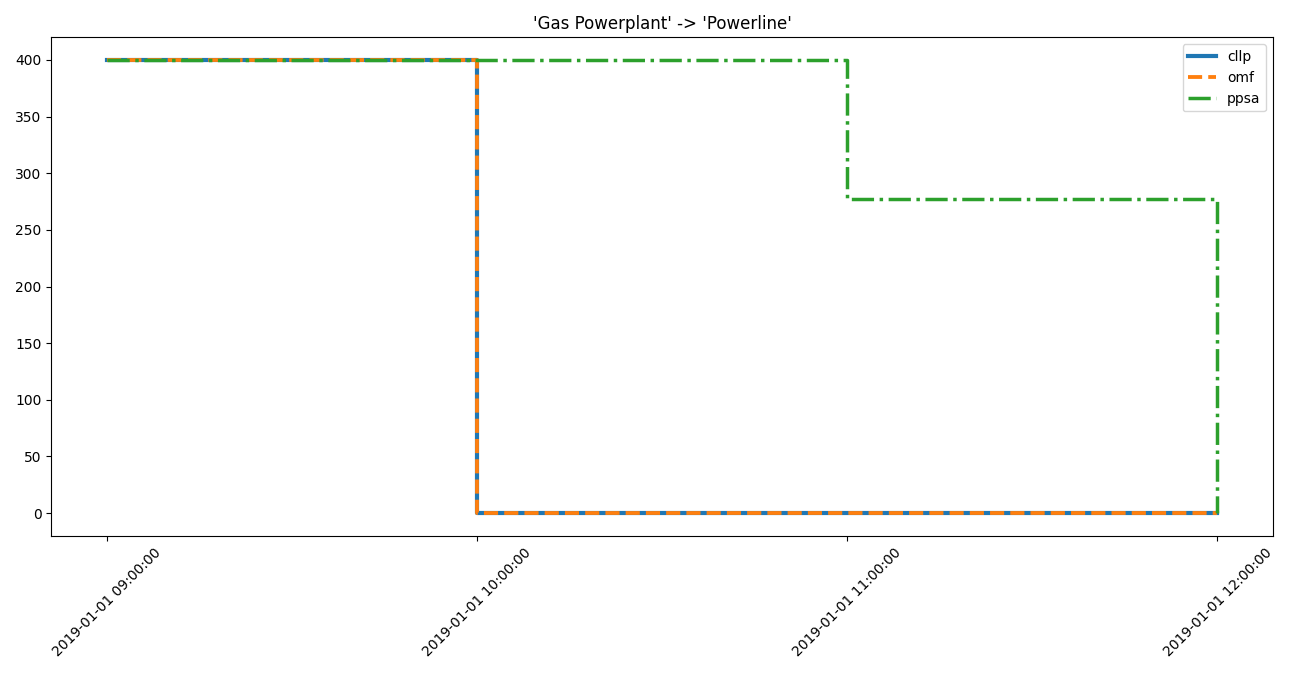
>>> for dtf in idf.high_interest_timeframes[('Gas Powerplant', 'Powerline')]:
... print(dtf)
... print(59*"-")
cllp omf ppsa
2019-01-01 09:00:00 400.0 400.0 400.00000
2019-01-01 10:00:00 0.0 0.0 400.00000
2019-01-01 11:00:00 0.0 0.0 277.13932
2019-01-01 12:00:00 0.0 0.0 0.00000
-----------------------------------------------------------
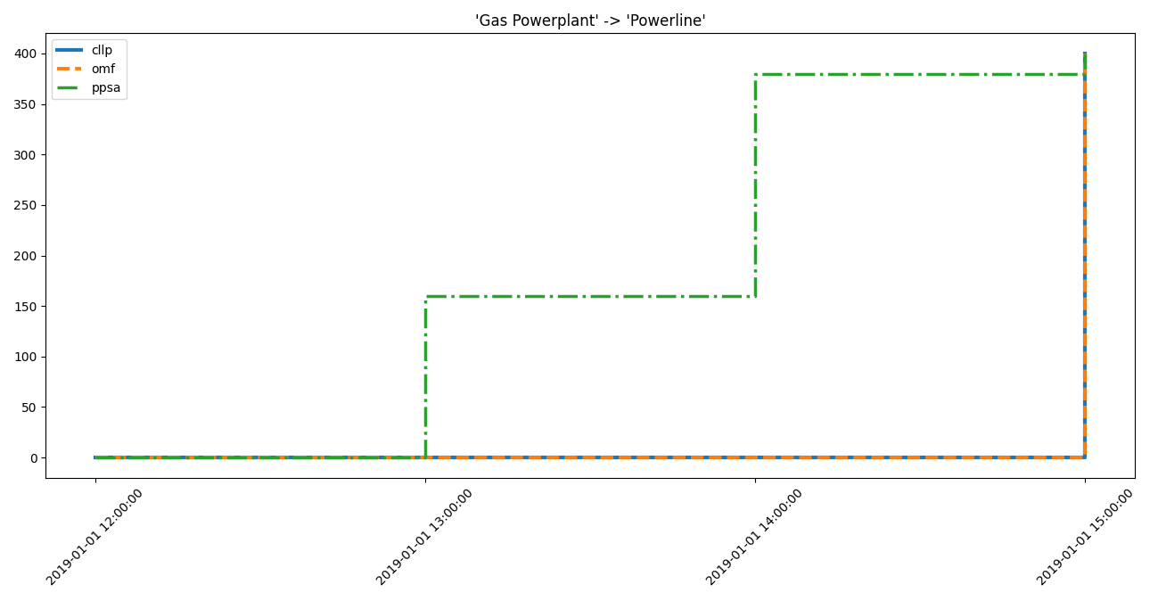
cllp omf ppsa
2019-01-01 12:00:00 0.0 0.0 0.0000
2019-01-01 13:00:00 0.0 0.0 159.9942
2019-01-01 14:00:00 0.0 0.0 379.5134
2019-01-01 15:00:00 400.0 400.0 400.0000
-----------------------------------------------------------
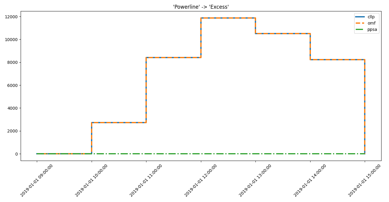
>>> for dtf in idf.high_interest_timeframes[('Powerline', 'Excess')]:
...     print(dtf)
                           cllp         omf  ppsa
2019-01-01 09:00:00      0.0000      0.0000   0.0
2019-01-01 10:00:00   2720.0957   2720.0957   0.0
2019-01-01 11:00:00   8413.8899   8413.8899   0.0
2019-01-01 12:00:00  11872.4380  11872.4380   0.0
2019-01-01 13:00:00  10502.7870  10502.7870   0.0
2019-01-01 14:00:00   8221.1174   8221.1174   0.0
2019-01-01 15:00:00      0.0000      0.0000   0.0
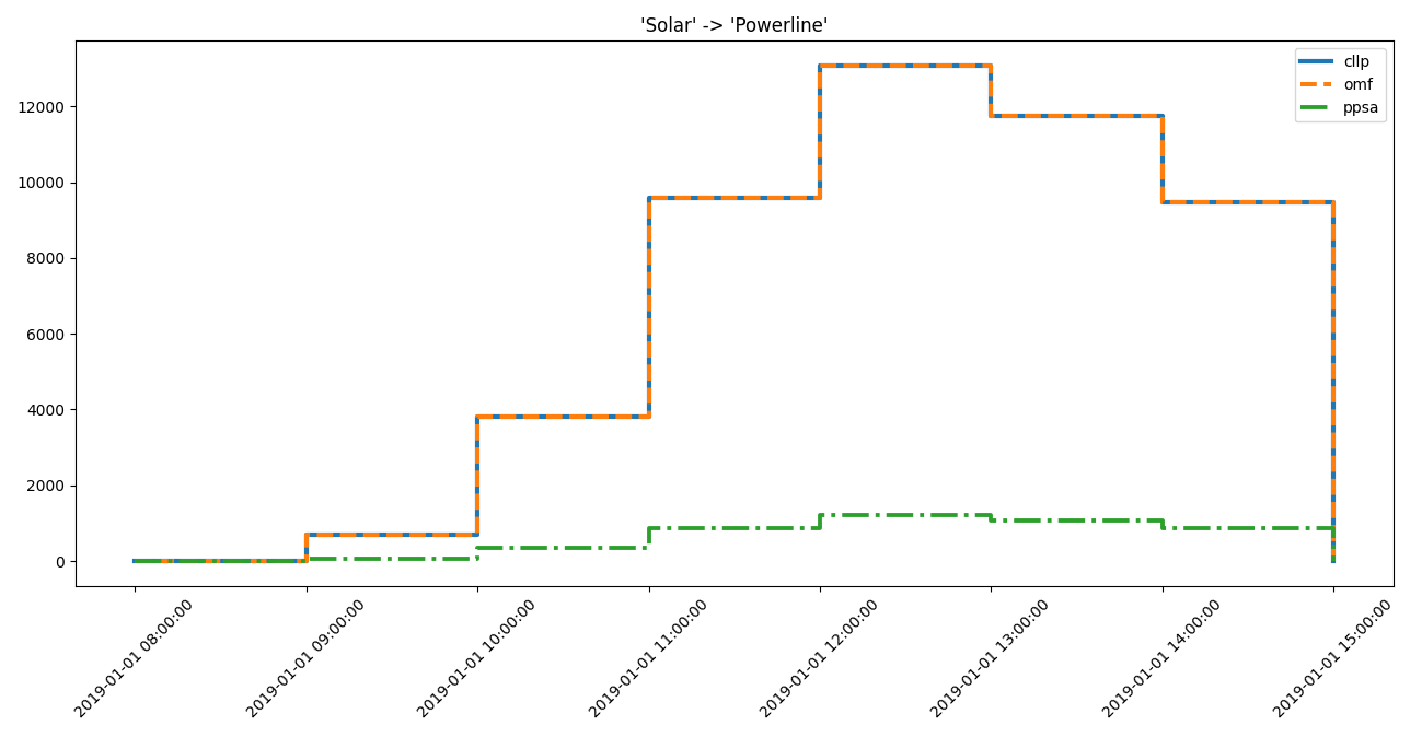
>>> for dtf in idf.medium_interest_timeframes[('Solar', 'Powerline')]:
...     print(dtf)
                           cllp         omf         ppsa
2019-01-01 08:00:00      0.0000      0.0000     0.000000
2019-01-01 09:00:00    680.6120    680.6120    62.645926
2019-01-01 10:00:00   3821.6497   3821.6497   351.758100
2019-01-01 11:00:00   9572.0769   9572.0769   881.047680
2019-01-01 12:00:00  13075.9990  13075.9990  1203.561000
2019-01-01 13:00:00  11743.7140  11743.7140  1080.932800
2019-01-01 14:00:00   9472.5144   9472.5144   871.883600
2019-01-01 15:00:00      0.0000      0.0000     0.000000
Use pandas.DataFrame.index if your really only interested in the actual
timeframes:
>>> for dtf in idf.medium_interest_timeframes[('Solar', 'Powerline')]:
...     print(dtf.index)
DatetimeIndex(['2019-01-01 08:00:00', '2019-01-01 09:00:00',
               '2019-01-01 10:00:00', '2019-01-01 11:00:00',
               '2019-01-01 12:00:00', '2019-01-01 13:00:00',
               '2019-01-01 14:00:00', '2019-01-01 15:00:00'],
              dtype='datetime64[ns]', freq=None)
Visualizing Timevarying Result Data of Identified Components and Narrowed Down Timeframes
Plotting the results for manual inspection:
>>> from tessif.visualize import component_loads
>>> for dtf in idf.high_interest_timeframes[('Gas Powerplant', 'Powerline')]:
...     axes = component_loads.step(dtf)
...     # axes.figure.show()  # commented out for doctesting
>>> from tessif.visualize import component_loads
>>> for dtf in idf.high_interest_timeframes[('Powerline', 'Excess')]:
...     axes = component_loads.step(dtf)
...     # axes.figure.show()  # commented out for doctesting
>>> from tessif.visualize import component_loads
>>> for dtf in idf.medium_interest_timeframes[('Solar', 'Powerline')]:
...     axes = component_loads.step(dtf)
...     # axes.figure.show()  # commented out for doctesting
Identifying Root Causes
The identificaiton of root causes is not subject of this tutorial. For further guidance, the respective phd thesis is recommended.
Used Utilities
Enerysystems to test timeseries algorithms
- tessif.examples.application.timeseries_comparison.create_hhes_ar(periods=24, directory=None, filename=None)[source]
Create a model of Hamburg’s energy system using
tessif's model.- Parameters:
periods¶ (int, default=24) – Number of time steps of the evaluated timeframe (one time step is one hour)
directory¶ (str, default=None) –
String representing of the path the created energy system is dumped to. Passed to
dump().Will be
joinedwithfilename.If set to
None(default)tessif.frused.paths.write_dir/tsf will be the chosen directory.filename¶ (str, default=None) –
dump()the energy system using this name.If set to
None(default) filename will behhes.tsf.
- Returns:
es – Tessif energy system.
- Return type:
References
Minimum Working Example - For a step by step explanation on how to create a Tessif energy system.
Hamburg Energy System Example (Brief) - For simulating and comparing this energy system using different supported models.
Examples
Use
create_hhes()to quickly access a tessif energy system to use for doctesting, or trying out this framework’s utilities.>>> import tessif.examples.data.tsf.py_hard as tsf_py >>> es = tsf_py.create_hhes()
>>> for node in es.nodes:
...     print(node.uid)
coal supply line
gas pipeline
oil supply line
waste supply
powerline
district heating pipeline
biomass logistics
gas supply
coal supply
oil supply
waste
pv1
won1
biomass supply
imported el
imported heat
demand el
demand th
excess el
excess th
chp1
chp2
chp3
chp4
chp5
chp6
pp1
pp2
pp3
pp4
hp1
p2h
biomass chp
est
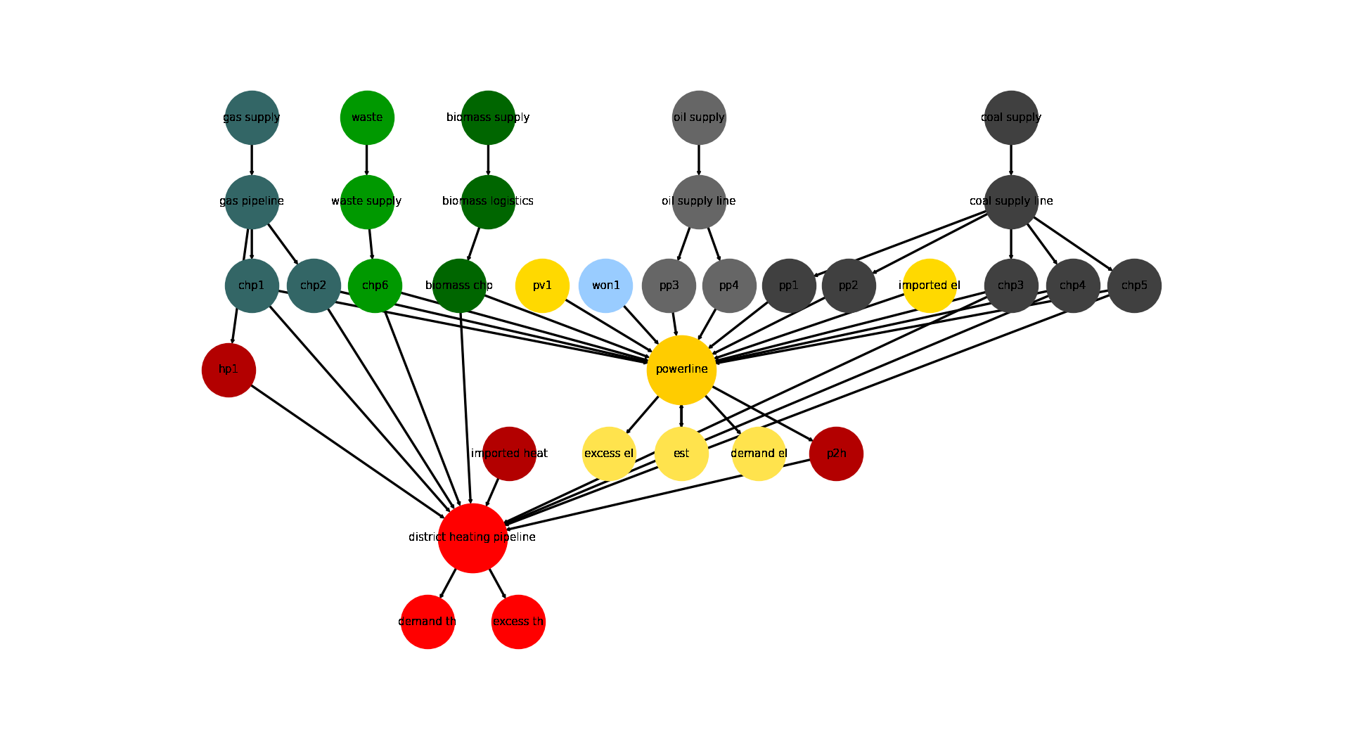
Visualize the energy system for better understanding what the output means:
>>> import matplotlib.pyplot as plt
>>> import tessif.visualize.nxgrph as nxv
>>> grph = es.to_nxgrph()
>>> drawing_data = nxv.draw_graph(
...     grph,
...     node_color={
...         'coal supply': '#404040',
...         'coal supply line': '#404040',
...         'pp1': '#404040',
...         'pp2': '#404040',
...         'chp3': '#404040',
...         'chp4': '#404040',
...         'chp5': '#404040',
...         'hp1': '#b30000',
...         'imported heat': '#b30000',
...         'district heating pipeline': 'Red',
...         'demand th': 'Red',
...         'excess th': 'Red',
...         'p2h': '#b30000',
...         'bm1': '#006600',
...         'won1': '#99ccff',
...         'gas supply': '#336666',
...         'gas pipeline': '#336666',
...         'chp1': '#336666',
...         'chp2': '#336666',
...         'waste': '#009900',
...         'waste supply': '#009900',
...         'chp6': '#009900',
...         'oil supply': '#666666',
...         'oil supply line': '#666666',
...         'pp3': '#666666',
...         'pp4': '#666666',
...         'pv1': '#ffd900',
...         'imported el': '#ffd900',
...         'demand el': '#ffe34d',
...         'excess el': '#ffe34d',
...         'est': '#ffe34d',
...         'powerline': '#ffcc00',
...     },
...     node_size={
...         'powerline': 5000,
...         'district heating pipeline': 5000
...     },
...     layout='dot',
... )
>>> # plt.show()  # commented out for simpler doctesting
- tessif.examples.application.timeseries_comparison.create_statistical_example_msc(periods=24)[source]
Create a model of Hamburg’s energy system using
tessif's model.- Parameters:
periods¶ (int, default=24) – Number of time steps of the evaluated timeframe (one time step is one hour)
- Returns:
es – Tessif energy system.
- Return type:
References
Minimum Working Example - For a step by step explanation on how to create a Tessif energy system.
Hamburg Energy System Example (Brief) - For simulating and comparing this energy system using different supported models.
Examples
Use
create_statistical_example_msc()to quickly access a tessif energy system model scenario combination (msc) to use for ting, or trying out this framework’s utilities:>>> from tessif.examples.application import timeseries_comparison >>> msc = timeseries_comparison.create_statistical_example_msc()
Visualize the msc as generic graph:
>>> import matplotlib.pyplot as plt
>>> import tessif.visualize.nxgrph as nxv
>>> drawing_data = nxv.draw_graph(
...     msc.to_nxgrph(),
...     node_color={
...        'Demand': '#ffe34d',
...        'Excess': '#ffe34d',
...        'Gas Supply': '#336666',
...        'Gas Pipeline': '#336666',
...        'Gas Powerplant': '#336666',
...        'Solar': '#FF7700',
...        'Powerline': '#ffcc00',
...        'Import': '#ffd900',
...     },
...     node_size={
...         'Powerline': 5000,
...     },
... )
>>> # plt.show()  # commented out for simpler doctesting