Calliope Integration Scenarios
For analysing the integration of Calliope into Tessif
some of the examples tessif.examples.data.tsf.py_hard have been adjusted to compare
even more parameters in detail.
These adjusted examples as well as some optimization results are given below.
Reference Energy Systems
Working Examples
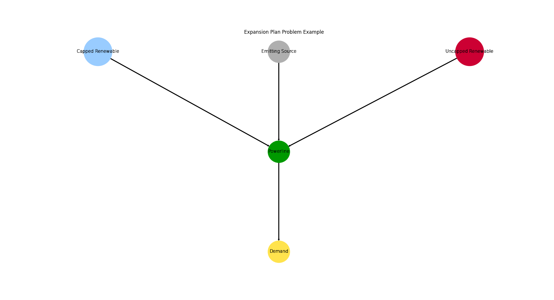
Create a small energy system utilizing two emisison free and expandable sources, as well as an emitting one. |
|
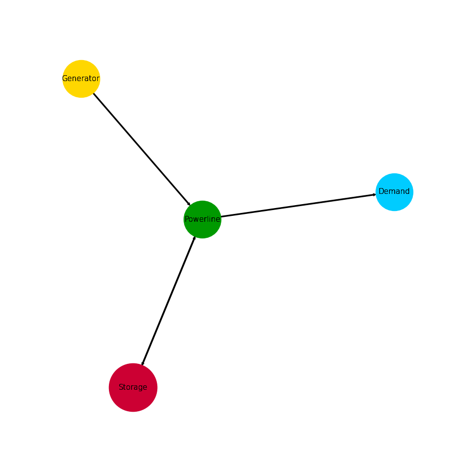
Create a small energy system utilizing an expandable storage with a fixed capacity to outflow ratio. |
|
Create a small energy system using |
|
Create a small energy system using |
|
Create a model of a generic component based energy system using |
calliope_integration_scenarios is a tessif
module aggregating the research results of a master thesis titled
Comparison of modelling tools to optimize energy systems via integration into
an existing framework for transforming energy system models
conducted by Max Reimer.
- tessif.examples.application.calliope_integration_scenarios.create_sources_example()[source]
Create a small energy system utilizing two emisison free and expandable sources, as well as an emitting one.
This small energy system was used to analyse the implementation of tessif sources, busses and demands in calliope as well as compare it to fine, oemof and pypsa. It is the same as the create_expansion_plan_example in
py_hard- Returns:
es – Tessif energy system.
- Return type:
Examples
Use
create_expansion_plan_example()to quickly access a tessif energy system to use for doctesting, or trying out this framework’s utilities.>>> import tessif.examples.application.calliope_integration_scenarios as examples >>> import matplotlib.pyplot as plt >>> import tessif.visualize.nxgrph as nxv >>> es = examples.create_sources_example() >>> grph = es.to_nxgrph() >>> drawing_data = nxv.draw_graph( ... grph, ... node_color={'Powerline': '#009900', ... 'Emitting Source': '#cc0033', ... 'Demand': '#00ccff', ... 'Capped Renewable': '#ffD700', ... 'Uncapped Renewable': '#ffD700',}, ... node_size={'Powerline': 5000}, ... layout='dot') >>> # plt.show() # commented out for simpler doctesting
- tessif.examples.application.calliope_integration_scenarios.create_storage_example()[source]
Create a small energy system utilizing an expandable storage with a fixed capacity to outflow ratio.
This small energy system was used to analyse the implementation of tessif storages in calliope as well as compare it to fine, oemof and pypsa. It is an adjusted model following the create_storage_fixed_ratio_expansion_example in
py_hard- Returns:
es – Tessif energy system.
- Return type:
Note
Calliope does not differ between input and outpuf efficiency, while the other tools do. Since this difference is already known analysing this is not needed anymore, hence the in and output efficiencies are set to be the same to find out unknown differences.
Examples
Using
create_storage_example()to quickly access a tessif energy system to use for doctesting, or trying out this frameworks utilities.>>> import tessif.examples.application.calliope_integration_scenarios as examples >>> import matplotlib.pyplot as plt >>> import tessif.visualize.nxgrph as nxv >>> tsf_es = examples.create_storage_example() >>> grph = tsf_es.to_nxgrph() >>> drawing_data = nxv.draw_graph( ... grph, ... node_color={'Powerline': '#009900', ... 'Storage': '#cc0033', ... 'Demand': '#00ccff', ... 'Generator': '#ffD700',}, ... node_size={'Storage': 5000}, ... layout='neato') >>> # plt.show() # commented out for simpler doctesting
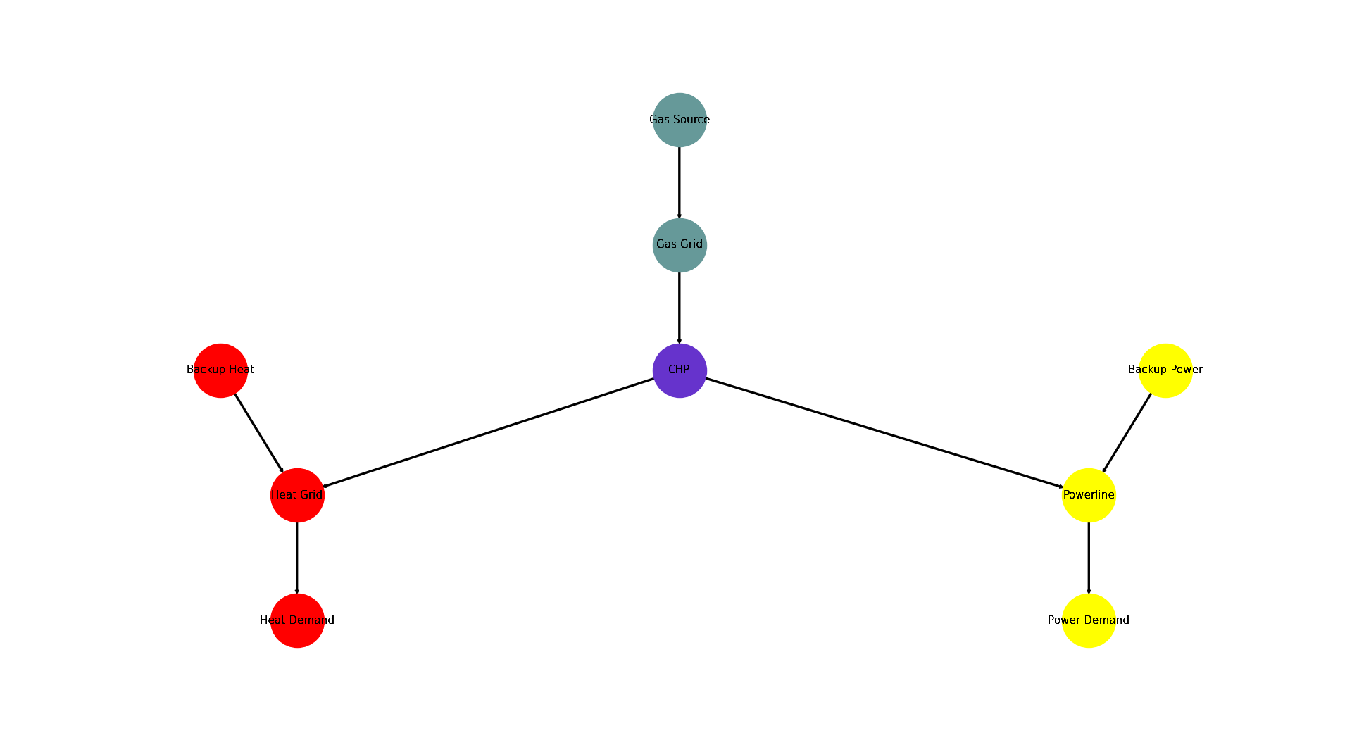
- tessif.examples.application.calliope_integration_scenarios.create_chp_example()[source]
Create a small energy system using
tessif's
model
optimizing it for costs to demonstrate a chp application.This small energy system was used to analyse the implementation of tessif multi output transformer in calliope as well as compare it to fine, oemof and pypsa. It is an adjusted model following the create_chp in
py_hard- Returns:
es – Tessif energy system.
- Return type:
Examples
Using
create_chp()to quickly access a tessif energy system to use for doctesting, or trying out this frameworks utilities.>>> import tessif.examples.application.calliope_integration_scenarios as examples >>> import matplotlib.pyplot as plt >>> import tessif.visualize.nxgrph as nxv >>> tsf_es = examples.create_chp_example() >>> grph = tsf_es.to_nxgrph() >>> drawing_data = nxv.draw_graph( ... grph, ... node_color={ ... 'Gas Source': '#669999', ... 'Gas Grid': '#669999', ... 'CHP': '#6633cc', ... 'Backup Heat': 'red', ... 'Heat Grid': 'red', ... 'Heat Demand': 'red', ... 'Backup Power': 'yellow', ... 'Powerline': 'yellow', ... 'Power Demand': 'yellow', ... }, ... ) >>> # plt.show() # commented out for simpler doctesting
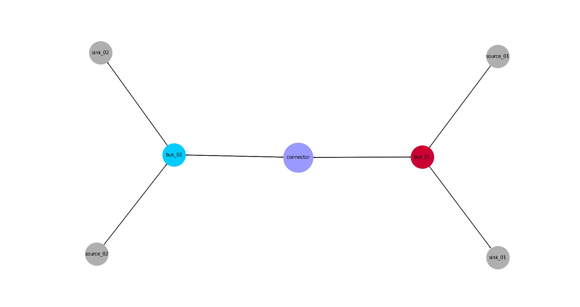
- tessif.examples.application.calliope_integration_scenarios.create_connector_example()[source]
Create a small energy system using
tessif's
model
optimizing it for costs to demonstrate a connector.This small energy system was used to analyse the implementation of tessif connector in calliope as well as compare it to fine, oemof and pypsa. It is an the same model as the create_connected_es in
py_hard- Returns:
es – Tessif energy system.
- Return type:
Examples
Using
create_connected_es()to quickly access a tessif energy system to use for doctesting, or trying out this frameworks utilities:>>> import tessif.examples.application.calliope_integration_scenarios as examples >>> import matplotlib.pyplot as plt >>> import tessif.visualize.nxgrph as nxv >>> es = examples.create_connector_example() >>> grph = es.to_nxgrph() >>> drawing_data = nxv.draw_graph( ... grph, ... node_color={'connector': '#9999ff', ... 'bus-01': '#cc0033', ... 'bus-02': '#00ccff'}, ... node_size={'connector': 5000}, ... layout='neato') >>> # plt.show() # commented out for simpler doctesting
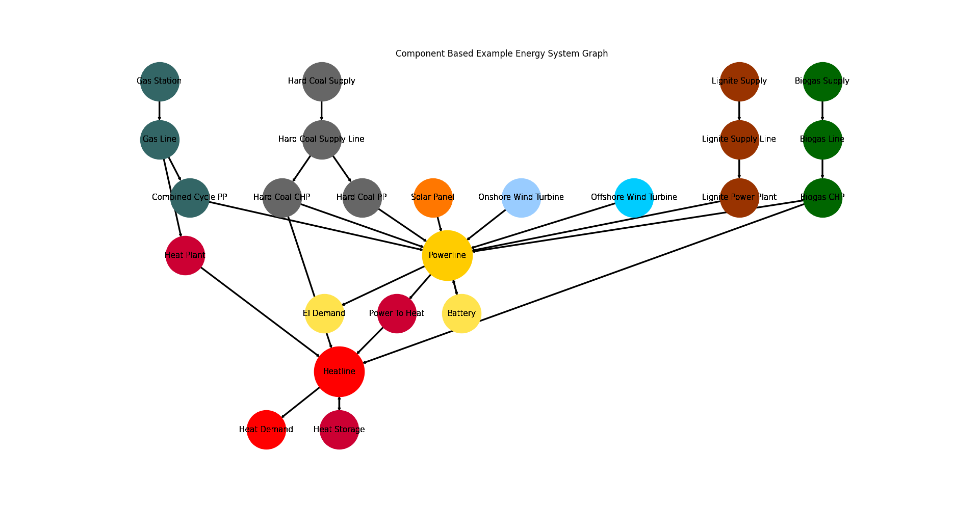
- tessif.examples.application.calliope_integration_scenarios.create_component_example(expansion_problem=False, periods=8760)[source]
Create a model of a generic component based energy system using
tessif's model.This energy system was used to compare calliope to fine, oemof and pypsa in a bigger example for the timeframe of a year in hourly resolution. It is an the same model as the create_component_es in
py_hard- Parameters:
- Returns:
es – Tessif energy system.
- Return type:
Examples
Use
create_component_es()to quickly access a tessif energy system to use for doctesting, or trying out this framework’s utilities.>>> import tessif.examples.application.calliope_integration_scenarios as examples >>> import matplotlib.pyplot as plt >>> import tessif.visualize.nxgrph as nxv >>> es = examples.create_component_example() >>> grph = es.to_nxgrph() >>> drawing_data = nxv.draw_graph( ... grph, ... node_color={ ... 'Hard Coal Supply': '#666666', ... 'Hard Coal Supply Line': '#666666', ... 'Hard Coal PP': '#666666', ... 'Hard Coal CHP': '#666666', ... 'Solar Panel': '#FF7700', ... 'Heat Storage': '#cc0033', ... 'Heat Demand': 'Red', ... 'Heat Plant': '#cc0033', ... 'Heatline': 'Red', ... 'Power To Heat': '#cc0033', ... 'Biogas CHP': '#006600', ... 'Biogas Line': '#006600', ... 'Biogas Supply': '#006600', ... 'Onshore Wind Turbine': '#99ccff', ... 'Offshore Wind Turbine': '#00ccff', ... 'Gas Station': '#336666', ... 'Gas Line': '#336666', ... 'Combined Cycle PP': '#336666', ... 'El Demand': '#ffe34d', ... 'Battery': '#ffe34d', ... 'Powerline': '#ffcc00', ... 'Lignite Supply': '#993300', ... 'Lignite Supply Line': '#993300', ... 'Lignite Power Plant': '#993300', ... }, ... node_size={ ... 'Powerline': 5000, ... 'Heatline': 5000 ... }, ... title='Component Based Example Energy System Graph', ... ) >>> # plt.show() # commented out for simpler doctesting
Optimization Results
Here the above listed example energy system are going to be used and analysed
aiming for the main differences of the modelling tools. Since this work has been done
after writing the calliope es2es.cllp and
es2mapping.cllp some differences are already known, like
calliope not being able to differ between storage input and output efficiency. These are
not further analysed in the here listed examples.
Analysing Sources, Demand and Busses
Import hardcoded tessif energy system as well as needed utilities
>>> import tessif.examples.application.calliope_integration_scenarios as examples
>>> import tessif.analyze
>>> import tessif.parse
>>> import os
>>> from tessif.frused.paths import write_dir
>>> import tessif.frused.configurations as configurations
>>> configurations.spellings_logging_level = 'debug'
Build and optimize the model with each of the (at the moment of this work) supported models
>>> tsf_es = examples.create_sources_example()
>>> output_msg = tsf_es.to_hdf5(
...     directory=os.path.join(write_dir, 'tsf'),
...     filename='comparison.hdf5',
... )
>>> comparatier = tessif.analyze.Comparatier(
...     path=os.path.join(write_dir, 'tsf', 'comparison.hdf5'),
...     parser=tessif.parse.hdf5,
...     models=('fine', 'calliope', 'pypsa', 'oemof'),
... )
Comparing optimization results
>>> for model in sorted(comparatier.models):
...     print(model)
cllp
fine
omf
ppsa
>>> print(comparatier.integrated_global_results)
                 cllp  fine   omf  ppsa
emissions (sim)  20.0  20.0  20.0  20.0
costs (sim)      41.0  41.0  41.0  41.0
opex (ppcd)      40.0  40.0  40.0  40.0
capex (ppcd)      1.0   1.0   1.0   1.0
time             15.0  15.0  15.0  15.0
memory           15.0  15.0  15.0  15.0
>>> for model in sorted(comparatier.models):
...     print(f'-  {model}  -')
...     print(comparatier.optimization_results[model].node_load['Powerline'])
-  cllp  -
Powerline            Capped Renewable  Emitting Source  Uncapped Renewable  Demand
1990-07-13 00:00:00             -3.25            -5.75                -1.0    10.0
1990-07-13 01:00:00             -3.25            -4.75                -2.0    10.0
1990-07-13 02:00:00             -3.25            -3.75                -3.0    10.0
1990-07-13 03:00:00             -3.25            -5.75                -1.0    10.0
-  fine  -
Powerline            Capped Renewable  Emitting Source  Uncapped Renewable  Demand
1990-07-13 00:00:00             -3.25            -5.75                -1.0    10.0
1990-07-13 01:00:00             -3.25            -4.75                -2.0    10.0
1990-07-13 02:00:00             -3.25            -3.75                -3.0    10.0
1990-07-13 03:00:00             -3.25            -5.75                -1.0    10.0
-  omf  -
Powerline            Capped Renewable  Emitting Source  Uncapped Renewable  Demand
1990-07-13 00:00:00             -3.25            -5.75                -1.0    10.0
1990-07-13 01:00:00             -3.25            -4.75                -2.0    10.0
1990-07-13 02:00:00             -3.25            -3.75                -3.0    10.0
1990-07-13 03:00:00             -3.25            -5.75                -1.0    10.0
-  ppsa  -
Powerline            Capped Renewable  Emitting Source  Uncapped Renewable  Demand
1990-07-13 00:00:00             -3.25            -5.75                -1.0    10.0
1990-07-13 01:00:00             -3.25            -4.75                -2.0    10.0
1990-07-13 02:00:00             -3.25            -3.75                -3.0    10.0
1990-07-13 03:00:00             -3.25            -5.75                -1.0    10.0
>>> print(comparatier.comparative_results.original_capacities['Capped Renewable'])
cllp    2.0
fine    2.0
omf     2.0
ppsa    2.0
Name: Capped Renewable, dtype: float64
>>> print(comparatier.comparative_results.original_capacities['Emitting Source'])
cllp    0.0
fine    0.0
omf     0.0
ppsa    0.0
Name: Emitting Source, dtype: float64
>>> print(comparatier.comparative_results.original_capacities['Uncapped Renewable'])
cllp    3.0
fine    3.0
omf     3.0
ppsa    3.0
Name: Uncapped Renewable, dtype: float64
The results on this example using three differently parameterized sources, a bus as well as a demand do stay the same no matter which tool is being used. Since the sources parameterization differs heavily and busses and demand usually aren’t very much parameterized at all, it can be assumed that all these three component types are implemented correctly and will most likely not lead to differences in other example energy systems.
Analysing Storage
Import hardcoded tessif energy system as well as needed utilities
>>> import tessif.examples.application.calliope_integration_scenarios as examples
>>> import tessif.analyze
>>> import tessif.parse
>>> import os
>>> from tessif.frused.paths import write_dir
>>> import tessif.frused.configurations as configurations
>>> configurations.spellings_logging_level = 'debug'
Build and optimize the model with each of the (at the moment of this work) supported models
>>> tsf_es = examples.create_storage_example()
>>> output_msg = tsf_es.to_hdf5(
...     directory=os.path.join(write_dir, 'tsf'),
...     filename='comparison.hdf5',
... )
>>> comparatier = tessif.analyze.Comparatier(
...     path=os.path.join(write_dir, 'tsf', 'comparison.hdf5'),
...     parser=tessif.parse.hdf5,
...     models=('fine', 'calliope', 'pypsa', 'oemof'),
... )
Comparing optimization results
>>> print(comparatier.integrated_global_results)
                  cllp   fine    omf   ppsa
emissions (sim)    8.0    8.0    8.0    8.0
costs (sim)      353.0  253.0  253.0  253.0
opex (ppcd)       15.0   15.0   15.0   15.0
capex (ppcd)     338.0  238.0  238.0  238.0
time              15.0   15.0   15.0   15.0
memory            15.0   15.0   15.0   15.0
>>> for model in sorted(comparatier.models):
...     print(f'-  {model}  -')
...     print(comparatier.optimization_results[model].node_load['Powerline'])
-  cllp  -
Powerline            Generator  Storage  Demand  Storage
1990-07-13 00:00:00      -19.0     -0.0    10.0      9.0
1990-07-13 01:00:00      -19.0     -0.0    10.0      9.0
1990-07-13 02:00:00      -19.0     -0.0     7.0     12.0
1990-07-13 03:00:00       -0.0     -5.0     5.0      0.0
1990-07-13 04:00:00       -0.0    -10.0    10.0      0.0
-  fine  -
Powerline            Generator  Storage  Demand  Storage
1990-07-13 00:00:00      -19.0     -0.0    10.0      9.0
1990-07-13 01:00:00      -19.0     -0.0    10.0      9.0
1990-07-13 02:00:00      -19.0     -0.0     7.0     12.0
1990-07-13 03:00:00       -0.0     -5.0     5.0      0.0
1990-07-13 04:00:00       -0.0    -10.0    10.0      0.0
-  omf  -
Powerline            Generator  Storage  Demand  Storage
1990-07-13 00:00:00      -19.0     -0.0    10.0      9.0
1990-07-13 01:00:00      -19.0     -0.0    10.0      9.0
1990-07-13 02:00:00      -19.0     -0.0     7.0     12.0
1990-07-13 03:00:00       -0.0     -5.0     5.0      0.0
1990-07-13 04:00:00       -0.0    -10.0    10.0      0.0
-  ppsa  -
Powerline            Generator  Storage  Demand  Storage
1990-07-13 00:00:00      -19.0     -0.0    10.0      9.0
1990-07-13 01:00:00      -19.0     -0.0    10.0      9.0
1990-07-13 02:00:00      -19.0     -0.0     7.0     12.0
1990-07-13 03:00:00       -0.0     -5.0     5.0      0.0
1990-07-13 04:00:00       -0.0    -10.0    10.0      0.0
>>> for stor in comparatier.comparative_results.socs:
...     print(comparatier.comparative_results.socs[stor])
Storage                    cllp     fine        omf       ppsa
1990-07-13 00:00:00   93.100000   0.0000  67.500000   8.595000
1990-07-13 01:00:00  100.269000   8.1000  74.925000  16.609050
1990-07-13 02:00:00  110.066310  16.1190  84.975750  27.242959
1990-07-13 03:00:00  103.410090  26.7578  78.570437  21.414974
1990-07-13 04:00:00   91.264879  20.9347  66.673621  10.089713
>>> print(comparatier.comparative_results.capacities['Storage'])
cllp    170.0
fine    120.0
omf     120.0
ppsa    120.0
Name: Storage, dtype: float64
The results of the storage example do differ the most. Calliope and oemof do refer the initial state of charge to the optimum capacity, while pypsa refers to the initial capacity and fine does not represent an initial SOC at all. Furthermore oemof and pypsa do take the storage loss into account starting from the initial SOC, while calliope starts one time step later. In addition calliope also has a different understanding of the flow rates. While the other tools limit the flow rate for input and output, calliope limits the maximum difference input to output difference of two successive timesteps. Thus the limit is 17 (12+5) and therefore a capacity of 170 is needed, since the flow rate is 10%.
Analysing Transformer
Import hardcoded tessif energy system as well as needed utilities
>>> import tessif.examples.application.calliope_integration_scenarios as examples
>>> import tessif.analyze
>>> import tessif.parse
>>> import os
>>> from tessif.frused.paths import write_dir
>>> import tessif.frused.configurations as configurations
>>> configurations.spellings_logging_level = 'debug'
Build and optimize the model with each of the (at the moment of this work) supported models
>>> tsf_es = examples.create_chp_example()
>>> output_msg = tsf_es.to_hdf5(
...     directory=os.path.join(write_dir, 'tsf'),
...     filename='comparison.hdf5',
... )
>>> comparatier = tessif.analyze.Comparatier(
...     path=os.path.join(write_dir, 'tsf', 'comparison.hdf5'),
...     parser=tessif.parse.hdf5,
...     models=('fine', 'calliope', 'pypsa', 'oemof'),
... )
Comparing optimization results
>>> print(comparatier.integrated_global_results)
                   cllp    fine     omf    ppsa
emissions (sim)   160.0   160.0   160.0   160.0
costs (sim)      1525.0  1525.0  1525.0  1525.0
opex (ppcd)      1506.0  1506.0  1506.0  1506.0
capex (ppcd)       19.0    19.0    19.0    19.0
time               15.0    15.0    15.0    15.0
memory             15.0    15.0    15.0    15.0
>>> for model in sorted(comparatier.models):
...     print(f'-  {model}  -')
...     print(comparatier.optimization_results[model].node_load['CHP'])
-  cllp  -
CHP                   Gas Grid  Heat Grid  Powerline
1990-07-13 00:00:00 -33.333333   6.666667       10.0
1990-07-13 01:00:00 -33.333333   6.666667       10.0
1990-07-13 02:00:00 -33.333333   6.666667       10.0
1990-07-13 03:00:00 -33.333333   6.666667       10.0
-  fine  -
CHP                   Gas Grid  Heat Grid  Powerline
1990-07-13 00:00:00 -33.333333   6.666667       10.0
1990-07-13 01:00:00 -33.333333   6.666667       10.0
1990-07-13 02:00:00 -33.333333   6.666667       10.0
1990-07-13 03:00:00 -33.333333   6.666667       10.0
-  omf  -
CHP                   Gas Grid  Heat Grid  Powerline
1990-07-13 00:00:00 -33.333333   6.666667       10.0
1990-07-13 01:00:00 -33.333333   6.666667       10.0
1990-07-13 02:00:00 -33.333333   6.666667       10.0
1990-07-13 03:00:00 -33.333333   6.666667       10.0
-  ppsa  -
CHP                   Gas Grid  Heat Grid  Powerline
1990-07-13 00:00:00 -33.333333   6.666667       10.0
1990-07-13 01:00:00 -33.333333   6.666667       10.0
1990-07-13 02:00:00 -33.333333   6.666667       10.0
1990-07-13 03:00:00 -33.333333   6.666667       10.0
>>> print(comparatier.comparative_results.original_capacities['CHP'])
CHP        cllp  fine  omf  ppsa
Heat Grid   2.0   2.0    2   2.0
Powerline   3.0   3.0    3   3.0
>>> print(comparatier.comparative_results.capacities['CHP'])
CHP             cllp    fine        omf       ppsa
Heat Grid   6.666667   6.667   6.666667   6.666667
Powerline  10.000000  10.000  10.000000  10.000000
>>> print(comparatier.comparative_results.expansion_costs['CHP'])
CHP            cllp  fine  omf  ppsa
Heat Grid  0.000000   1.0    1   1.0
Powerline  2.666667   2.0    2   2.0
>>> for edge in comparatier.comparative_results.emissions:
...     if edge.source == 'CHP':
...         print(comparatier.comparative_results.emissions[edge])
cllp    0.0
fine    3.0
omf     3.0
ppsa    3.0
Name: (CHP, Heat Grid), dtype: float64
cllp    4.0
fine    2.0
omf     2.0
ppsa    2.0
Name: (CHP, Powerline), dtype: float64
The overall results do stay the same no matter which tools is used. But calliope can only refer emissions and costs to one output carrier, thus this minor difference can be seen when going in detail on the costs and emissions.
Analysing Connector
Import hardcoded tessif energy system as well as needed utilities
>>> import tessif.examples.application.calliope_integration_scenarios as examples
>>> import tessif.analyze
>>> import tessif.parse
>>> import os
>>> from tessif.frused.paths import write_dir
>>> import tessif.frused.configurations as configurations
>>> configurations.spellings_logging_level = 'debug'
Build and optimize the model with each of the (at the moment of this work) supported models
>>> tsf_es = examples.create_connector_example()
>>> output_msg = tsf_es.to_hdf5(
...     directory=os.path.join(write_dir, 'tsf'),
...     filename='comparison.hdf5',
... )
>>> comparatier = tessif.analyze.Comparatier(
...     path=os.path.join(write_dir, 'tsf', 'comparison.hdf5'),
...     parser=tessif.parse.hdf5,
...     models=('fine', 'calliope', 'pypsa', 'oemof'),
... )
Comparing optimization results
>>> for model in sorted(comparatier.models):
...     print(f'-  {model}  -')
...     print(comparatier.optimization_results[model].node_load['bus-01'])
...     print(comparatier.optimization_results[model].node_load['bus-02'])
-  cllp  -
bus-01               connector  source-01  connector  sink-01
1990-07-13 00:00:00       -0.0  -5.555556   5.555556      0.0
1990-07-13 01:00:00       -5.0 -10.000000   0.000000     15.0
1990-07-13 02:00:00       -0.0 -10.000000   0.000000     10.0
bus-02               connector  source-02  connector  sink-02
1990-07-13 00:00:00       -5.0     -10.00       0.00     15.0
1990-07-13 01:00:00       -0.0      -6.25       6.25      0.0
1990-07-13 02:00:00       -0.0     -10.00       0.00     10.0
-  fine  -
bus-01               connector  source-01  connector  sink-01
1990-07-13 00:00:00       -0.0  -5.555556   5.555556      0.0
1990-07-13 01:00:00       -5.0 -10.000000   0.000000     15.0
1990-07-13 02:00:00       -0.0 -10.000000   0.000000     10.0
bus-02               connector  source-02  connector  sink-02
1990-07-13 00:00:00       -5.0     -10.00       0.00     15.0
1990-07-13 01:00:00       -0.0      -6.25       6.25      0.0
1990-07-13 02:00:00       -0.0     -10.00       0.00     10.0
-  omf  -
bus-01               connector  source-01  connector  sink-01
1990-07-13 00:00:00       -0.0  -5.555556   5.555556      0.0
1990-07-13 01:00:00       -5.0 -10.000000   0.000000     15.0
1990-07-13 02:00:00       -0.0 -10.000000   0.000000     10.0
bus-02               connector  source-02  connector  sink-02
1990-07-13 00:00:00       -5.0     -10.00       0.00     15.0
1990-07-13 01:00:00       -0.0      -6.25       6.25      0.0
1990-07-13 02:00:00       -0.0     -10.00       0.00     10.0
-  ppsa  -
bus-01               connector  source-01  connector  sink-01
1990-07-13 00:00:00       -0.0       -5.0        5.0      0.0
1990-07-13 01:00:00      -10.0       -5.0        0.0     15.0
1990-07-13 02:00:00       -0.0      -10.0        0.0     10.0
bus-02               connector  source-02  connector  sink-02
1990-07-13 00:00:00       -5.0      -10.0        0.0     15.0
1990-07-13 01:00:00       -0.0      -10.0       10.0      0.0
1990-07-13 02:00:00       -0.0      -10.0        0.0     10.0
Pypsa remains the only tool not being able to represent the tessif connectors efficiencies.
Analysing Component Example
Commitment Scenario
Import hardcoded tessif energy system as well as needed utilities
>>> import tessif.examples.application.calliope_integration_scenarios as examples
>>> import tessif.analyze
>>> import tessif.parse
>>> import os
>>> from tessif.frused.paths import write_dir
>>> import tessif.frused.configurations as configurations
>>> configurations.spellings_logging_level = 'debug'
Build and optimize the model with each of the (at the moment of this work) supported models
>>> tsf_es = examples.create_component_example(periods=8760)
>>> output_msg = tsf_es.to_hdf5(
...     directory=os.path.join(write_dir, 'tsf'),
...     filename='comparison.hdf5',
... )
>>> comparatier = tessif.analyze.Comparatier(
...     path=os.path.join(write_dir, 'tsf', 'comparison.hdf5'),
...     parser=tessif.parse.hdf5,
...     models=('fine', 'calliope', 'pypsa', 'oemof'),
... )
Comparing optimization results
>>> print(comparatier.integrated_global_results)
                        cllp         fine          omf         ppsa
emissions (sim)    6982535.0    6815288.0    6813556.0    6833502.0
costs (sim)      688509348.0  688509319.0  688509325.0  688509325.0
opex (ppcd)      688509352.0  688509319.0  688509325.0  688509325.0
capex (ppcd)             0.0          0.0          0.0          0.0
time                    15.0         15.0         15.0         15.0
memory                  15.0         15.0         15.0         15.0
>>> loads_of_interest = dict(cllp=dict(), fine=dict(), omf=dict(), ppsa=dict())
>>> for key in comparatier.comparative_results.loads['Powerline'].sum().keys():
...     tool = key[0]
...     for component, value in comparatier.comparative_results.loads['Powerline'].sum()[tool].items():
...         if value != 0:
...             loads_of_interest[tool].update({f'{component}': comparatier.comparative_results.loads['Powerline'].sum()['ppsa'][component]})
>>> import pprint
>>> pprint.pprint(loads_of_interest)
{'cllp': {'Combined Cycle PP': -31949.064820970012,
          'El Demand': 9809506.139999973,
          'Hard Coal CHP': -1107094.3751364017,
          'Hard Coal PP': -2094456.862612009,
          'Lignite Power Plant': -4132599.8522110027,
          'Onshore Wind Turbine': -2081332.7192399953,
          'Solar Panel': -362073.2661429987},
 'fine': {'Combined Cycle PP': -31949.064820970012,
          'El Demand': 9809506.139999973,
          'Hard Coal CHP': -1107094.3751364017,
          'Hard Coal PP': -2094456.862612009,
          'Lignite Power Plant': -4132599.8522110027,
          'Onshore Wind Turbine': -2081332.7192399953,
          'Solar Panel': -362073.2661429987},
 'omf': {'Combined Cycle PP': -31949.064820970012,
         'El Demand': 9809506.139999973,
         'Hard Coal CHP': -1107094.3751364017,
         'Hard Coal PP': -2094456.862612009,
         'Lignite Power Plant': -4132599.8522110027,
         'Onshore Wind Turbine': -2081332.7192399953,
         'Solar Panel': -362073.2661429987},
 'ppsa': {'Combined Cycle PP': -31949.064820970012,
          'El Demand': 9809506.139999973,
          'Hard Coal CHP': -1107094.3751364017,
          'Hard Coal PP': -2094456.862612009,
          'Lignite Power Plant': -4132599.8522110027,
          'Onshore Wind Turbine': -2081332.7192399953,
          'Solar Panel': -362073.2661429987}}
Apart from the emission difference due to different emission at same cost from the solar panel and the hard coal power plant, the differences in costs are very small.
Expansion Scenario
Import hardcoded tessif energy system as well as needed utilities
>>> import tessif.examples.application.calliope_integration_scenarios as examples
>>> import tessif.analyze
>>> import tessif.parse
>>> import os
>>> from tessif.frused.paths import write_dir
>>> import tessif.frused.configurations as configurations
>>> configurations.spellings_logging_level = 'debug'
Build and optimize the model with each of the (at the moment of this work) supported models
>>> tsf_es = examples.create_component_example(periods=8760, expansion_problem=True)
>>> output_msg = tsf_es.to_hdf5(
...     directory=os.path.join(write_dir, 'tsf'),
...     filename='comparison.hdf5',
... )
>>> comparatier = tessif.analyze.Comparatier(
...     path=os.path.join(write_dir, 'tsf', 'comparison.hdf5'),
...     parser=tessif.parse.hdf5,
...     models=('fine', 'calliope', 'pypsa', 'oemof'),
... )
Comparing optimization results
>>> print(comparatier.integrated_global_results)
                         cllp          fine           omf          ppsa
emissions (sim)  2.500000e+05  2.500000e+05  2.500000e+05  2.655080e+05
costs (sim)      4.228912e+10  4.228912e+10  4.228912e+10  3.772778e+10
opex (ppcd)      7.342042e+08  7.341404e+08  7.341404e+08  8.230078e+08
capex (ppcd)     4.155492e+10  4.155498e+10  4.155498e+10  3.690477e+10
time             1.500000e+01  1.500000e+01  1.500000e+01  1.500000e+01
memory           1.500000e+01  1.500000e+01  1.500000e+01  1.500000e+01
It can be seen that the calliope results are pretty much the same
as the fine and oemof results. The results for pypsa are deeply analysed
in component_scenarios and
thus not being analysed here again.
Timeseries aggregation
Import hardcoded tessif energy system as well as needed utilities
>>> import tessif.examples.application.calliope_integration_scenarios as examples
>>> import tessif.analyze
>>> import tessif.parse
>>> import os
>>> from tessif.frused.paths import write_dir
>>> import tessif.frused.configurations as configurations
>>> configurations.spellings_logging_level = 'debug'
Build and optimize the model with each of the (at the moment of this work) supported models
>>> step_size = [6, 12, 18, 24, ]
>>> results = dict()
>>> for i in step_size:
...     tsf_es = examples.create_component_example(periods=8760, expansion_problem=False)
...     output_msg = tsf_es.to_hdf5(
...         directory=os.path.join(write_dir, 'tsf'),
...         filename='comparison.hdf5',
...     )
...     comparatier = tessif.analyze.Comparatier(
...         path=os.path.join(write_dir, 'tsf', 'comparison.hdf5'),
...         parser=tessif.parse.hdf5,
...         models=('calliope',),
...         trans_ops={'calliope': {'aggregate': i}}
...     )
...     results[f'{i}'] = dict(comparatier.integrated_global_results)
>>> for key,res in results.items():
...     print(key)
...     print(res)
...     print(79*'-')
step_size_6
{'cllp': capex (ppcd)               0.0
costs (sim)        688013068.0
emissions (sim)      6997381.0
memory                    15.0
opex (ppcd)        688013071.0
time                      15.0
Name: cllp, dtype: float64}
-------------------------------------------------------------------------------
step_size_12
{'cllp': capex (ppcd)               0.0
costs (sim)        687286213.0
emissions (sim)      7084048.0
memory                    15.0
opex (ppcd)        687286211.0
time                      15.0
Name: cllp, dtype: float64}
-------------------------------------------------------------------------------
step_size_18
{'cllp': capex (ppcd)               0.0
costs (sim)        686957383.0
emissions (sim)      7087157.0
memory                    15.0
opex (ppcd)        686957380.0
time                      15.0
Name: cllp, dtype: float64}
-------------------------------------------------------------------------------
step_size_24
{'cllp': capex (ppcd)               0.0
costs (sim)        686756663.0
emissions (sim)      7102717.0
memory                    15.0
opex (ppcd)        686756664.0
time                      15.0
Name: cllp, dtype: float64}
-------------------------------------------------------------------------------
>>> step_size = [6, 12, 18, 24, ]
>>> results = dict()
>>> for i in step_size:
...     tsf_es = examples.create_component_example(periods=8760, expansion_problem=True)
...     output_msg = tsf_es.to_hdf5(
...         directory=os.path.join(write_dir, 'tsf'),
...         filename='comparison.hdf5',
...     )
...     comparatier = tessif.analyze.Comparatier(
...         path=os.path.join(write_dir, 'tsf', 'comparison.hdf5'),
...         parser=tessif.parse.hdf5,
...         models=('calliope',),
...         trans_ops={'calliope': {'aggregate': i}}
...     )
...     results[f'{i}'] = dict(comparatier.integrated_global_results)
>>> for key,res in results.items():
...     print(key)
...     print(res)
...     print(79*'-')
6
{'cllp': capex (ppcd)       3.893490e+10
costs (sim)        3.966113e+10
emissions (sim)    2.500000e+05
memory             1.500000e+01
opex (ppcd)        7.262305e+08
time               1.500000e+01
Name: cllp, dtype: float64}
-------------------------------------------------------------------------------
12
{'cllp': capex (ppcd)       3.245386e+10
costs (sim)        3.316322e+10
emissions (sim)    2.500000e+05
memory             1.500000e+01
opex (ppcd)        7.093545e+08
time               1.500000e+01
Name: cllp, dtype: float64}
-------------------------------------------------------------------------------
18
{'cllp': capex (ppcd)       2.767016e+10
costs (sim)        2.840622e+10
emissions (sim)    2.500000e+05
memory             1.500000e+01
opex (ppcd)        7.360632e+08
time               1.500000e+01
Name: cllp, dtype: float64}
-------------------------------------------------------------------------------
24
{'cllp': capex (ppcd)       2.733419e+10
costs (sim)        2.803969e+10
emissions (sim)    2.500000e+05
memory             1.500000e+01
opex (ppcd)        7.055088e+08
time               1.500000e+01
Name: cllp, dtype: float64}
-------------------------------------------------------------------------------
The timeseries aggregation for both examples shows lower expected costs with higher step sizes.
Used Utilities
calliope_integration_scenarios is a tessif
module aggregating the research results of a master thesis titled
Comparison of modelling tools to optimize energy systems via integration into
an existing framework for transforming energy system models
conducted by Max Reimer.