Comparative Result Analysis

As identified in the Preliminary Result Analysis, the Component Expansion and the modified Component Expansion model scenario combinations, are deemed to be subject to a detailed comparative result analysis. Following subsections aim to identify key differences between the softwares investigated, as well as to locate root causes from which these differences originate.

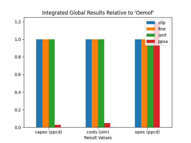
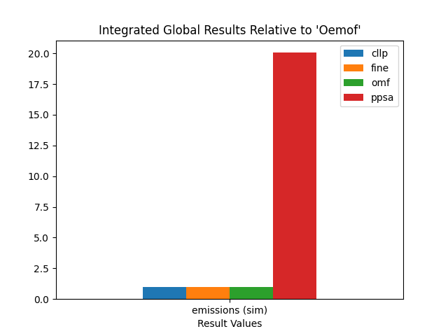
High Priority Results / Integrated Global Results

CompE

IGR [€ or t_CO2]	cllp	fine	omf	ppsa
capex (ppcd)	41554917514	41554976118	41554977878	1132235997
costs (sim)	42289121225	42289118279	42289118239	2062636560
emissions (sim)	250000	250000	250000	5014819
opex (ppcd)	734204228	734140364	734140364	874603138

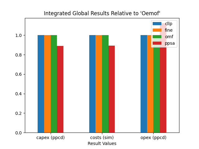
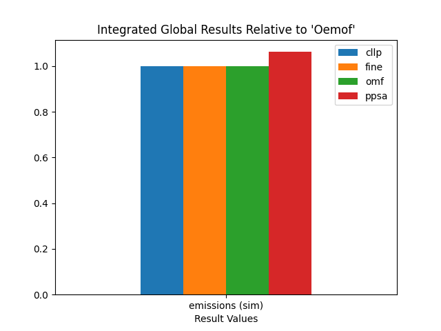
Modified CompE

IGR [€ or t_CO2]	cllp	fine	omf	ppsa
capex (ppcd)	41554917514	41554976118	41554977878	36904768288
costs (sim)	42289121225	42289118279	42289118239	37727776780
emissions (sim)	250000	250000	250000	265508
opex (ppcd)	734204228	734140364	734140364	823007841

Advanced Graph / Advanced System Visualization

The advanced graph / advanced system visualizations (AGV / ASV respectively) of the preselected model-scenario combinations (MSCs) are shown below. A list of relevant observations is made further below in the respective ISD sections when perfroming the visual comparison.

The AGS subsection closes with some additional remarks on what observations are considered to be helpful in an investigation focused on the actual results rather than their comparison. It also serves demonstration purposes on how to use the AVS and the benefits it brings.

Component Expansion (CompE)

Oemof

PyPSA

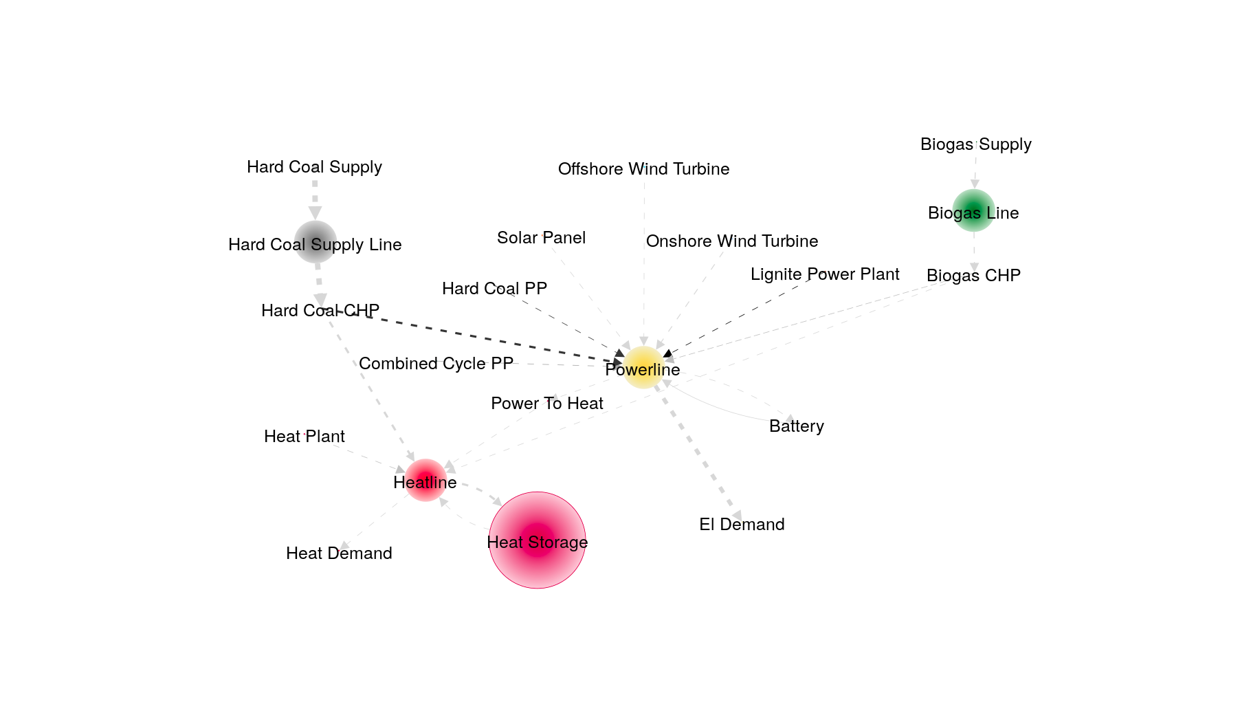
The Preliminary Result Analysis indicates, that the PyPSA results differ significantly. An initial attempt to relate node size to the installed capacity and net energy flow of the demand component 'El Demand' fails, since the resulting size of the Heat Storage component is too large. Thus the advanced system visualization below is plotted, relating node size to the installed capacity of the Heat Storage component.

Modified Component Expansion (Modified CompE)

Modifying the PyPSA system model scenario combination, leads to optimization results closer to that of the other softwares. The advanced graph below is therfor again drawn relative to the installed capacity and net energy flow of the demand component 'El Demand'.

PyPSA

Actual Result Analysis

When using the advanced graph / advanced system visualization for analysing the results as would be the case in actual research / investigations, following information can be exctracted:

1. For the optimal solution the components Onshore, Solar, Offshore and 'Battery' and Heat Storage are used the most, having relatively large installed capacities compared to the relatively low characteristic value / capacity factor.

2. The Onshore component supplies most of the power, as indicated by the arrow width.

3. Most of the heat is supplied by the power2heat component, as again, indicated by the arrow width.

4. All technologies used have relatively low specific emissions, as indicated by the light grey of the arrows of significant width.

5. All of the controllable power plant components ('Lignite PP', 'Hard Coal PP', 'Hard Coal CHP', 'Hard Coal CHP' and 'Combined Cycle PP') have an installed capacity greater than zero but only very litte to no use, as indicated by the combination of node size and node fill size.

Identifying Significant Differences

Findings of the identifying significant differences (ISD) step, part of the comparative results analysis are laid out and discussed in the following. As argued in the Preliminary Result Analysis, only the CompE and Modified CompE results are subject to the ISD method. The following explanation thereby serve the purpose of detecting the differences as well as to showcase the method itself and its features.

Components of Interest

Identification of the components of interest (COI), is the first step. In case a preliminary result analysis was performed like in this field study, components causing the differences might be already identified or at least hinted at. If not, which is usually the case for large system models, they are identified using the technologies below.

Visual Comparison

Using the advanced graph / advanced system visualization (AGV / ASV respectively), in conjunction with the integrated global results (IGR) visualization for quickly spotting few major differences and formulating hypotheses on their relations, even in large system models, is possible. For cases however, where there are many large differences (e.g. the CompE model scenario combination (MSC)), or barely any difference at all (e.g. The CompC MSC), visually comparing the ASVs and IGRs of different software tools can be of no benefit. For the two MSCs selected by the Preliminary Result Analysis however, the observations are listed below.

Component Expansion (CompE)

Comparing the above 'Oemof advanced graph visulaizations to the PyPSA one from below, following observations can be made:

1. The "Onshore Wind Turbine component is used for most of the energy supplied as indicated by the arrow width.

2. Specific emissions of the 'Heat Storage' is seemingly in the same order of magnitude for both software tools, as indicated by the arrow greyscale.

Following observations of the PyPSA advanced graph and integrated global results visulaizations were made:

1. The non-modified expansion combination of PyPSA differs largely in comparison to Oemof.

2. The 'Biogas' and 'Hard Coal' commodities are used for most of the energy supplied as indicated by the respective arrow widths.

3. The 'Hard Coal CHP' and the 'Biogas CHP' comonent are used for providing most of the power and heat as indicated by the arrow width.

4. The 'Hard Coal CHP' component causes significant amounts of emissions indicated by arrow width and blackness.

5. The total amount of integrated global emissions is comparaively very high, as seen by the bar size.

6. The 'Heat Storage' component is used extensively as indicated by node size and node fill size.

7. Comparaively, the Onshore Wind Turbine, Solar, Offshore Wind Turbine and 'Power To Heat' components are used far less.

Modified Component Expansion (Modified CompE)

Comparing the advanced graph visualization of the modified PyPSA component expansion model scenario combination, following aspects can be identified:

1. The modified PyPSA visualization resembles that of Oemof much closer in comparison to the non-modified variation.

2. The installed capacity of the 'Battery' component is larger, as indicated by the node size

Statistical Identifciation

In addition to the visaully enhanced manual inspection, the developed method propses a statistical identifciation technique, which is made accessible via the tessif.identify submodule. Findings and additional insights are presented below, categoriezed by investigated model scenario combination.

For both combinations the entirety of the statistical identifciation results is shown for purposes of demonstration. If, in an application context, the desired output are only certain levels of interest, those can be accessed easily via the respective interest keys word (i.e ‘high’ for ‘of-high-interest’ etc.). Examples of this can be found in the digital addendum and the respective online documentation.

Component Expansion (CompE)

The tables below list the identified levels of interest for both the timevarying load results and the static installed capacity results. In addition, the auxilliary results of calculated correlation coefficients and error value results as well as the relative deviation results are given to showcase internal usage of the method implementation. All of the tables shown are directly accessible via their respective interfaces of the tessif.identify submodule.

Identifciation of significantly deviating load results:

		cllp	fine	omf	ppsa
Battery	Powerline	low	low	low	high
Biogas CHP	Heatline	low	low	low	high
Biogas CHP	Powerline	low	low	low	high
Biogas Line	Biogas CHP	low	low	low	high
Biogas Supply	Biogas Line	low	low	low	high
Combined Cycle PP	Powerline	low	low	low	high
Hard Coal CHP	Heatline	None	None	None	high
Hard Coal CHP	Powerline	None	None	None	high
Hard Coal PP	Powerline	None	None	None	None
Hard Coal Supply	Hard Coal Supply Line	None	None	None	high
Hard Coal Supply Line	Hard Coal CHP	None	None	None	high
Heat Plant	Heatline	None	None	None	None
Heat Storage	Heatline	low	low	low	high
Heatline	Heat Demand	low	low	low	low
Heatline	Heat Storage	low	low	low	high
Lignite Power Plant	Powerline	None	None	None	None
Offshore Wind Turbine	Powerline	low	low	low	high
Onshore Wind Turbine	Powerline	low	low	low	high
Power To Heat	Heatline	low	low	low	high
Powerline	Battery	low	low	low	high
Powerline	El Demand	low	low	low	low
Powerline	Power To Heat	low	low	low	high
Solar Panel	Powerline	low	low	low	high

Calculated correlations:

		cllp	fine	omf	ppsa
Battery	Powerline	1.0	1.0	1.0	0.03
Biogas CHP	Heatline	1.0	1.0	1.0	0.14
Biogas CHP	Powerline	1.0	1.0	1.0	0.14
Biogas Line	Biogas CHP	1.0	1.0	1.0	0.14
Biogas Supply	Biogas Line	1.0	1.0	1.0	0.14
Combined Cycle PP	Powerline	1.0	1.0	1.0	0.23
Hard Coal CHP	Heatline	0.0	0.0	0.0	0.0
Hard Coal CHP	Powerline	0.0	0.0	0.0	0.0
Hard Coal PP	Powerline	0.0	0.0	0.0	0.0
Hard Coal Supply	Hard Coal Supply Line	0.0	0.0	0.0	0.0
Hard Coal Supply Line	Hard Coal CHP	0.0	0.0	0.0	0.0
Heat Plant	Heatline	0.0	0.0	0.0	0.0
Heat Storage	Heatline	1.0	1.0	1.0	-0.0
Heatline	Heat Demand	1.0	1.0	1.0	1.0
Heatline	Heat Storage	1.0	1.0	1.0	0.1
Lignite Power Plant	Powerline	0.0	0.0	0.0	0.0
Offshore Wind Turbine	Powerline	1.0	1.0	1.0	-0.16
Onshore Wind Turbine	Powerline	1.0	1.0	1.0	0.52
Power To Heat	Heatline	1.0	1.0	1.0	0.0
Powerline	Battery	1.0	1.0	1.0	-0.01
Powerline	El Demand	1.0	1.0	1.0	1.0
Powerline	Power To Heat	1.0	1.0	1.0	0.0
Solar Panel	Powerline	1.0	1.0	1.0	0.35

Calculated error values:

		cllp	fine	omf	ppsa
Battery	Powerline	0.01	0.0	0.0	1.26
Biogas CHP	Heatline	0.0	0.0	0.0	13.54
Biogas CHP	Powerline	0.0	0.0	0.0	13.54
Biogas Line	Biogas CHP	0.0	0.0	0.0	13.54
Biogas Supply	Biogas Line	0.0	0.0	0.0	13.54
Combined Cycle PP	Powerline	0.02	0.0	0.0	39.15
Hard Coal CHP	Heatline	None	None	None	inf
Hard Coal CHP	Powerline	None	None	None	inf
Hard Coal PP	Powerline	None	None	None	None
Hard Coal Supply	Hard Coal Supply Line	None	None	None	inf
Hard Coal Supply Line	Hard Coal CHP	None	None	None	inf
Heat Plant	Heatline	None	None	None	None
Heat Storage	Heatline	0.0	0.0	0.0	1.0
Heatline	Heat Demand	0.0	0.0	0.0	0.0
Heatline	Heat Storage	0.0	0.0	0.0	37.63
Lignite Power Plant	Powerline	None	None	None	None
Offshore Wind Turbine	Powerline	0.0	0.0	0.0	1.68
Onshore Wind Turbine	Powerline	0.0	0.0	0.0	0.81
Power To Heat	Heatline	0.0	0.0	0.0	1.0
Powerline	Battery	0.0	0.0	0.0	1.26
Powerline	El Demand	0.0	0.0	0.0	0.0
Powerline	Power To Heat	0.0	0.0	0.0	1.0
Solar Panel	Powerline	0.0	0.0	0.0	3.22

Identifciation of significantly deviating capacity results:

	cllp	fine	omf	ppsa
Battery	low	low	low	high
Biogas CHP Heatline	low	low	low	high
Biogas CHP Powerline	low	low	low	high
Biogas Supply	low	low	low	high
Combined Cycle PP	low	low	low	low
El Demand	low	low	low	low
Gas Station	low	low	low	None
Hard Coal CHP Heatline	low	low	low	high
Hard Coal CHP Powerline	low	low	low	high
Hard Coal PP	low	low	low	low
Hard Coal Supply	None	None	None	high
Heat Demand	low	low	low	low
Heat Plant	low	low	low	low
Heat Storage	low	low	low	high
Lignite Power Plant	low	low	low	low
Lignite Supply	None	None	None	None
Offshore Wind Turbine	low	low	low	high
Onshore Wind Turbine	low	low	low	high
Power To Heat	low	low	low	high
Solar Panel	low	low	low	high

Calculated deviations:

	cllp	fine	omf	ppsa
Battery	0.0	0.0	0.0	0.95
Biogas CHP Heatline	0.01	0.0	0.0	0.61
Biogas CHP Powerline	0.01	0.0	0.0	0.61
Biogas Supply	0.01	0.0	0.0	0.61
Combined Cycle PP	0.0	0.0	0.0	0.0
El Demand	0.0	0.0	0.0	0.0
Gas Station	0.01	0.0	0.0	None
Hard Coal CHP Heatline	0.0	0.0	0.0	1.1
Hard Coal CHP Powerline	0.0	0.0	0.0	1.1
Hard Coal PP	0.0	0.0	0.0	0.0
Hard Coal Supply	None	None	None	inf
Heat Demand	0.0	0.0	0.0	0.0
Heat Plant	0.0	0.0	0.0	0.0
Heat Storage	0.01	0.0	0.0	9.06
Lignite Power Plant	0.0	0.0	0.0	0.0
Lignite Supply	None	None	None	None
Offshore Wind Turbine	0.0	0.0	0.0	0.94
Onshore Wind Turbine	0.0	0.0	0.0	0.93
Power To Heat	0.0	0.0	0.0	0.83
Solar Panel	0.0	0.0	0.0	0.71

As indicated in (paragraph of method description chapter), standard parameterization of the statistical identification tools is not suited well, for isolating singular occurences in a comparison where many large differences exist. Hence this analysis does not provide any further key insights other than confirming already observed aspects:

1. PyPSA uses the 'Biogas' and 'Hard Coal' commodities and their subsequent transformer technologies, very differently, as indicated by level of interest, correlation coefficients and relative deviations of the installed capacities.

2. PyPSA usage differences of the 'Heat Storage' component are very very large as indicated by relative deviation of the installed capacities (9.06) and the correlation coefficient of the respective load results (0.1).

3. PyPSA utilizes the Onshore Wind Turbine, Solar, Offshore Wind Turbine and 'Power To Heat' components very differently.

One additional aspect however, gets highlighted by the statistical identifciation, that is difficult to detect, using the bar charts of the CompE alone, since the actual bar length is quite small:

3. PyPSA also uses the 'Battery' component very differently as indicated by relative deviation of the installed capacity (0.95) and the correlation coefficient of the respective load results (0.03).

Modified Component Expansion (Modified CompE)

Listed below, are the tables showing the identification results of the modified Component-Expansion model-scenario-combination. As before, all results including calculated correlations, error-values and relative deviations are shown to demonstrate their usage.

Identifciation of significantly deviating load results:

		cllp	fine	omf	ppsa
Battery	Powerline	low	low	low	high
Biogas CHP	Heatline	low	low	low	medium
Biogas CHP	Powerline	low	low	low	medium
Biogas Line	Biogas CHP	low	low	low	medium
Biogas Supply	Biogas Line	low	low	low	medium
Combined Cycle PP	Powerline	low	low	low	medium
Hard Coal CHP	Heatline	None	None	None	None
Hard Coal CHP	Powerline	None	None	None	None
Hard Coal PP	Powerline	None	None	None	None
Hard Coal Supply	Hard Coal Supply Line	None	None	None	None
Hard Coal Supply Line	Hard Coal CHP	None	None	None	None
Heat Plant	Heatline	None	None	None	None
Heat Storage	Heatline	low	low	low	medium
Heatline	Heat Demand	low	low	low	low
Heatline	Heat Storage	low	low	low	high
Lignite Power Plant	Powerline	None	None	None	None
Offshore Wind Turbine	Powerline	low	low	low	medium
Onshore Wind Turbine	Powerline	low	low	low	low
Power To Heat	Heatline	low	low	low	medium
Powerline	Battery	low	low	low	high
Powerline	El Demand	low	low	low	low
Powerline	Power To Heat	low	low	low	medium
Solar Panel	Powerline	low	low	low	medium

Calculated correlations:

		cllp	fine	omf	ppsa
Battery	Powerline	1.0	1.0	1.0	0.59
Biogas CHP	Heatline	1.0	1.0	1.0	0.93
Biogas CHP	Powerline	1.0	1.0	1.0	0.93
Biogas Line	Biogas CHP	1.0	1.0	1.0	0.93
Biogas Supply	Biogas Line	1.0	1.0	1.0	0.93
Combined Cycle PP	Powerline	1.0	1.0	1.0	0.95
Hard Coal CHP	Heatline	0.0	0.0	0.0	0.0
Hard Coal CHP	Powerline	0.0	0.0	0.0	0.0
Hard Coal PP	Powerline	0.0	0.0	0.0	0.0
Hard Coal Supply	Hard Coal Supply Line	0.0	0.0	0.0	0.0
Hard Coal Supply Line	Hard Coal CHP	0.0	0.0	0.0	0.0
Heat Plant	Heatline	0.0	0.0	0.0	0.0
Heat Storage	Heatline	1.0	1.0	1.0	0.8
Heatline	Heat Demand	1.0	1.0	1.0	1.0
Heatline	Heat Storage	1.0	1.0	1.0	0.61
Lignite Power Plant	Powerline	0.0	0.0	0.0	0.0
Offshore Wind Turbine	Powerline	1.0	1.0	1.0	0.73
Onshore Wind Turbine	Powerline	1.0	1.0	1.0	0.93
Power To Heat	Heatline	1.0	1.0	1.0	0.81
Powerline	Battery	1.0	1.0	1.0	0.17
Powerline	El Demand	1.0	1.0	1.0	1.0
Powerline	Power To Heat	1.0	1.0	1.0	0.81
Solar Panel	Powerline	1.0	1.0	1.0	0.86

Calculated error values:

		cllp	fine	omf	ppsa
Battery	Powerline	0.01	0.0	0.0	3.17
Biogas CHP	Heatline	0.0	0.0	0.0	0.38
Biogas CHP	Powerline	0.0	0.0	0.0	0.38
Biogas Line	Biogas CHP	0.0	0.0	0.0	0.38
Biogas Supply	Biogas Line	0.0	0.0	0.0	0.38
Combined Cycle PP	Powerline	0.02	0.0	0.0	0.6
Hard Coal CHP	Heatline	None	None	None	None
Hard Coal CHP	Powerline	None	None	None	None
Hard Coal PP	Powerline	None	None	None	None
Hard Coal Supply	Hard Coal Supply Line	None	None	None	None
Hard Coal Supply Line	Hard Coal CHP	None	None	None	None
Heat Plant	Heatline	None	None	None	None
Heat Storage	Heatline	0.0	0.0	0.0	0.53
Heatline	Heat Demand	0.0	0.0	0.0	0.0
Heatline	Heat Storage	0.0	0.0	0.0	1.17
Lignite Power Plant	Powerline	None	None	None	None
Offshore Wind Turbine	Powerline	0.0	0.0	0.0	0.77
Onshore Wind Turbine	Powerline	0.0	0.0	0.0	0.05
Power To Heat	Heatline	0.0	0.0	0.0	0.18
Powerline	Battery	0.0	0.0	0.0	4.4
Powerline	El Demand	0.0	0.0	0.0	0.0
Powerline	Power To Heat	0.0	0.0	0.0	0.18
Solar Panel	Powerline	0.0	0.0	0.0	0.51

Identifciation of significantly deviating capacity results:

	cllp	fine	omf	ppsa
Battery	low	low	low	high
Biogas CHP Heatline	low	low	low	medium
Biogas CHP Powerline	low	low	low	medium
Biogas Supply	low	low	low	medium
Combined Cycle PP	low	low	low	low
El Demand	low	low	low	low
Gas Station	low	low	low	None
Hard Coal CHP Heatline	low	low	low	low
Hard Coal CHP Powerline	low	low	low	low
Hard Coal PP	low	low	low	low
Hard Coal Supply	None	None	None	None
Heat Demand	low	low	low	low
Heat Plant	low	low	low	low
Heat Storage	low	low	low	low
Lignite Power Plant	low	low	low	low
Lignite Supply	None	None	None	None
Offshore Wind Turbine	low	low	low	medium
Onshore Wind Turbine	low	low	low	medium
Power To Heat	low	low	low	medium
Solar Panel	low	low	low	low

Calculated deviations:

	cllp	fine	omf	ppsa
Battery	-0.0	0.0	0.0	0.79
Biogas CHP Heatline	0.01	-0.0	0.0	-0.15
Biogas CHP Powerline	0.01	-0.0	0.0	-0.15
Biogas Supply	0.01	-0.0	0.0	-0.15
Combined Cycle PP	0.0	0.0	0.0	0.0
El Demand	0.0	0.0	0.0	0.0
Gas Station	-0.01	-0.0	0.0	None
Hard Coal CHP Heatline	0.0	0.0	0.0	0.0
Hard Coal CHP Powerline	0.0	0.0	0.0	0.0
Hard Coal PP	0.0	0.0	0.0	0.0
Hard Coal Supply	None	None	None	None
Heat Demand	-0.0	0.0	0.0	0.0
Heat Plant	0.0	0.0	0.0	0.0
Heat Storage	0.01	0.0	0.0	-0.02
Lignite Power Plant	0.0	0.0	0.0	0.0
Lignite Supply	None	None	None	None
Offshore Wind Turbine	0.0	-0.0	0.0	-0.17
Onshore Wind Turbine	-0.0	0.0	0.0	-0.2
Power To Heat	-0.0	0.0	0.0	0.1
Solar Panel	0.0	-0.0	0.0	-0.03

As indicated by the preliminary result analysis, the 'Battery' component of PyPSA might be responsible for the observed deviations in global integrated emissions. Using the proposed statistical identifciation technique, following points are to be observed:

1. The 'Battery' component of PyPSA is expanded much more than in the other softwares. Indicated during preliminary result analysis (figure XYZ) and confirmed here by level of interest (table XYZ) and relative deviation (0.79 table XYZ) of the installed capacities.

2. PyPSA uses its 'Battery' component similar to the other softwares when discharging, as indicated by the still relatively high correlation coefficient (0.59 table XYZ).

2. PyPSA uses its 'Battery' component quite differently to the other softwares when storing power, as indicated by the still relatively low correlation coefficient (0.17 table).

4. The amount of energy transferred from and to the 'Battery' component of PyPSA differs substantially compared to the remaining software tools as indicated by the calculated, relative deviation values of 3.17 and 4.40 for discharging and charging, respectively.

5. Same tendencies, but not as obvious, are noteable with the 'Heat Storage' component of PyPSA. With the discharging results even only beeing of ‘medium’ interest according to the identifciation.

6. Deviations of ‘medium’ interest, as identified, includes the low emitting components Onshore Wind Turbine, Offshore Wind Turbine and Solar as well as the higher emitting but less expensive components 'Biogas CHP' and 'Combined Cycle PP', as indicated by the level of intrerest results for both the timevarying load results (table XYZ) as well as the static installed capacity results (table XYZ).

Differing Timeframes

Identifying differing timeframes, as proposed by the respective method description, is most useful in cases where the actual results are subject of primary interest. In a comparative analysis for the sake of comparison, as done in this thesis however, they are most ofen of subordinate significance. Since major differences, leading to educated assumptions of root casues, can be made without comparing the actual timevarying results. Which is shown by the component identifciation above and the hypotheses formulation below.

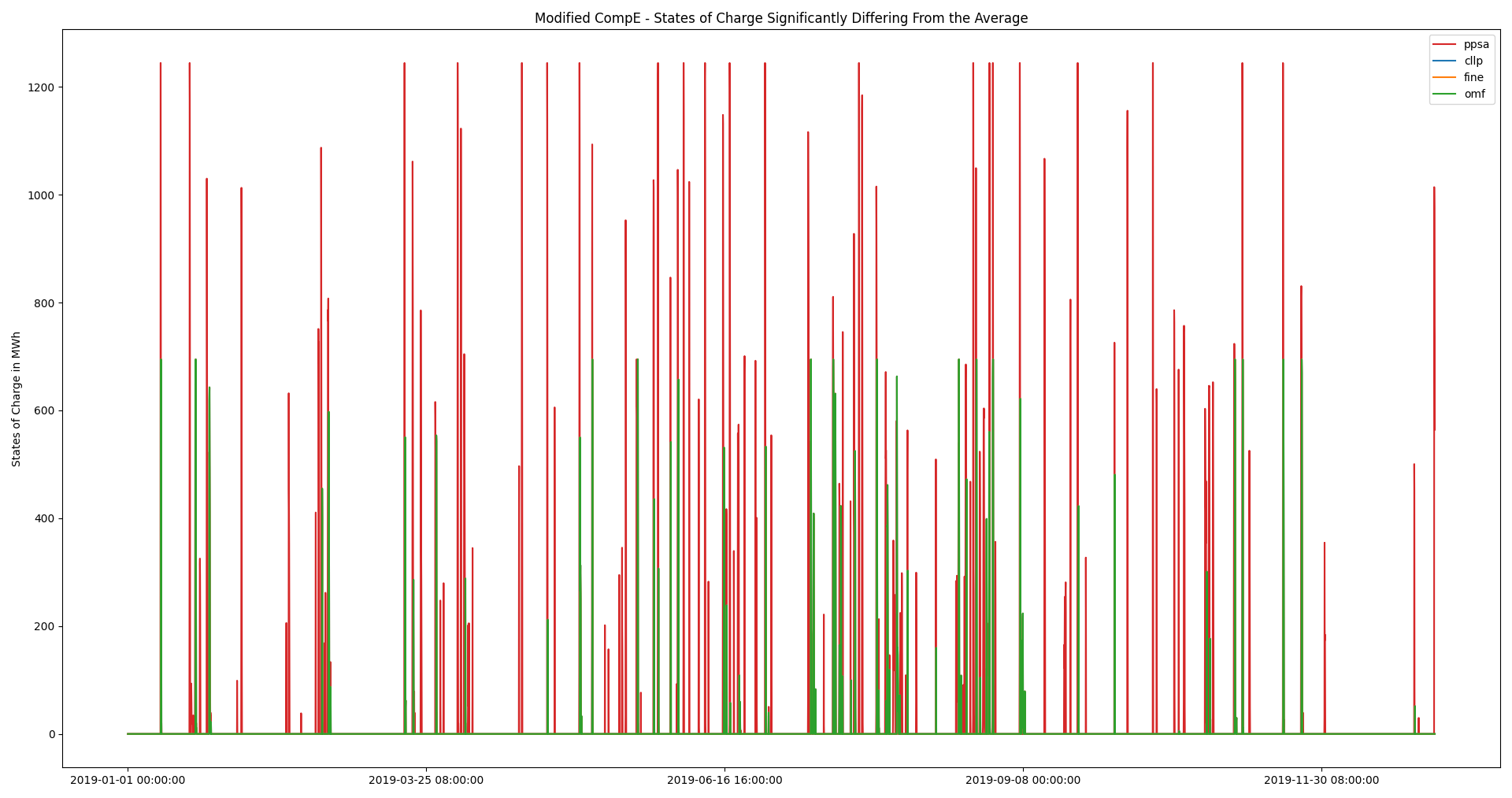
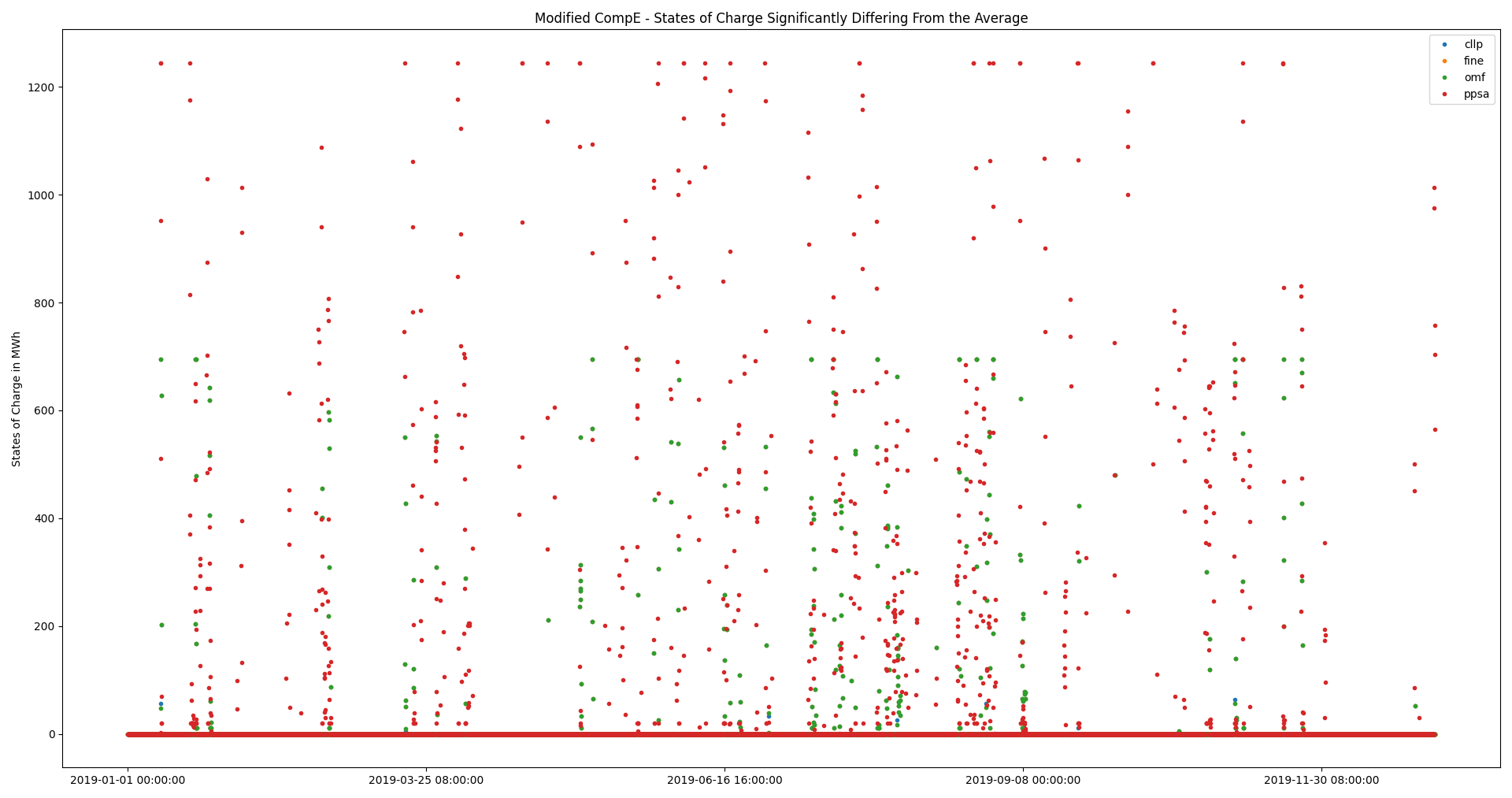
For purposes of demonstration, the first start and end points of the identified timeframes as well as examplary visualization of above-threshold timevarying result differences, for the flow from the 'Powerline' component to the 'Battery', are shown in the table and figures below. The SOC visualization at the bottom plots each SOC as a dot to highlight the identified deviations.

Index Number	(Start, End)
0	(‘2019-01-10 01:00:00’, ‘2019-01-10 10:00:00’)
1	(‘2019-01-18 04:00:00’, ‘2019-01-18 11:00:00’)
2	(‘2019-01-18 16:00:00’, ‘2019-01-19 05:00:00’)
3	(‘2019-01-19 05:00:00’, ‘2019-01-19 10:00:00’)
4	(‘2019-01-19 17:00:00’, ‘2019-01-20 05:00:00’)
5	(‘2019-01-21 01:00:00’, ‘2019-01-21 07:00:00’)
6	(‘2019-01-22 23:00:00’, ‘2019-01-23 09:00:00’)

Further Analysis Selection

After identifying differing components and timeframes, both visually as well as statistically, conclusions are drawn which potential root causes should be investigated further.

Component Expansion (CompE)

Hypotheses formulated based on the visual and statistical identification analysis performed above:

1. The emissions caused by the 'Hard Coal CHP' component of PyPSA are probably higher than intendend. Most likely beeing part of the reason, for why integrated global emissions differ as much.

2. The 'Hard Coal CHP' and 'Biogas CHP' components of PyPSA are used to provide most of the power and heat. This, in conjunction with the comparaively very high installed capacity of the 'Heat Storage' component, further indicate chp related emissions allocation issues, probably leading to large amounts of unneded thermal energy, that is stored inside the heat storage. Potentially indicating that no cyclic state of charge constraint is used, as intended by tessif’s parameterization.

3. The identified differences of the Onshore Wind Turbine, Solar, Offshore Wind Turbine and 'Power To Heat' component are probably only a result of the above, since they are parameterized as overall less cost efficient. Leading the solver to not use them, if possible despite the emission constraint.

Hence following questions are suggested to beeing answered by identifying potential root causes:

1. Do the PyPSA CHP components respect the allocated emissions as intended by Tessif?

2. Is there substantial amount of unused thermal energy inside the heat storage?

3. Does PyPSA use a non-cyclic state of charge constraint and is it the same for all of the software tools?

Modified Component Expansion (Modified CompE)

Hypotheses formulated based on the visual and statistical identification analysis performed above:

1. Energy flow specific emissions for the 'Battery' component are likely to be within the same order of magnitude between 'oemof' and 'PyPSA', yet the PyPSA time integrated global emission results are higher. Since PyPSA installed capacity of the 'Battery' comonent is comparatively larger, this indicates remaining differences in storage component emissions allocations.

2. Similar conclusions can be drawn on the 'Heat Storage' component further indicating a systematic difference of storage components between 'PyPSA' and the other software tools.

3. The observed shift in power generation from less emitting to less expensive but more emitting technologies by PyPSA compared to the other softwares are most likely a result of the interpreted, lower storage component emissions.

Based on the formulated hypotheses, following question is suggested to beeing answered during the identifciation of root causes:

• Do the PyPSA storage components interpret allocated emissions the same way as the other software tools?

Identifying Root Causes

During the ISD Analysis several questions were worked out to be answered during the identifying root causes (IRC) analysis. In the following they are listed again and rephased slightly (if necessary) to match the more general nature of the IRC analysis:

1. Do the PyPSA CHP components respect the allocated emissions as intended by Tessif? And how does that compare to the other software tools?

2. Is there substantial amount of unused thermal energy inside the heat storage for the CompE MSC? Implying that PyPSA uses the non-cyclic state-of-charge constraint as implied by Tessif. How does it compare to the other software tools?

3. Do the PyPSA storage components interpret allocated emissions the same way as the other software tools?

Suggesting following investigations:

1. CHP components and emissions:

   1. Perform a tabular-parameter-comparison of the CompE MSC 'Hard Coal CHP' to check an emission parameter exists and is allocated correctly.

   2. Perform a plausiblity check using a small system model focused around a singular chp component, imposing an emission constraint forcing the solver to use more expansive, but less emitting alternatives.

2. Storage components and cyclic state-of-charge constriants:

   1. Perform a tabular-parameter-comparison of the CompE MSC 'Heat Storage' component to check a cycle state-of-charge parameter exits and is allocated correctly.

   2. Perform a plausbility check, using a small system model focused around a singular storage component, not imposing a cyclic state-of-charge constraint, while making it less expensive to produce surplus amounts of energy that just get stored inside the storage and not used.

   3. Plot the timevarying state of charge results of all storage components of the CompE MSC to check for large amounts of unused thermal energy as part of ‘checking leftover ISD hypotheses’ like described in the respective IRC subsection.

3. Storage components and emissions:

   1. Perform a tabular-parameter-comparison of the CompE MSC 'Heat Storage' component to check an emission parameter exists and is allocated correctly.

   2. Perform a plausbility check, using a small system model focused around a singular storage component having outflow allocated emissions, a cyclic state-of-charge constraint while also having a more expensive, but less emitting alternative.

CHP Components and Emissions

Parameter Analysis

Parameter	Tessif	PyPSA
Component	Transformer	Generator (Link)
Identifier	Uid	name
Connecting Input(s)	inputs	(bus0)
Connecting Output(s)	outputs	bus (bus1)
Conversion Factors	conversions	(efficiency)
Energy Flow Specific Flow Cost	flow_costs	marginal_cost
Energy Flow Specific Emissions	flow emissions
Minimum Capacity	flow_rates.min	p_min_pu * p_nom
Maximum Capacity	flow_rates.max	p_max_pu * p_nom
Load Profile	timeseries	p_set

• Tabular Parameter Comparison shows that PyPSA CHP component does not have an inherent emission allocation parameter.

• PyPSa Doku states: “Global constraints are added to OPF problems and apply to many components at once. Currently only constraints related to primary energy (i.e. before conversion with losses by generators) are supported, the canonical example being CO2 emissions for an optimisation period. Other primary-energy-related gas emissions also fall into this framework.”

• Tessif circumvents that by adding an individual carrier to its PyPSA networks for each component having co2 emissions allocated, as for examples stated by the Tessif Doku: “Note how an extra Carrier object gets parsed to accomodate for the Link allocated emission constraints.”

• Tessifs intended parameters show emission allocation:

  Parameter	Parameter Values
  conversions	{(‘Hard_Coal’, ‘electricity’): 0.4, (‘Hard_Coal’, ‘hot_water’): 0.4}
  costs_for_being_active	0.0
  expandable	{‘Hard_Coal’: False, ‘electricity’: True, ‘hot_water’: True}
  expansion_costs	{‘Hard_Coal’: 0, ‘electricity’: 1750000, ‘hot_water’: 131250}
  expansion_limits	{‘Hard_Coal’: MinMax(min=0, max=inf), ‘electricity’: MinMax(min=300, max=inf), ‘hot_water’: MinMax(min=300, max=inf)}
  flow_costs	{‘Hard_Coal’: 0, ‘electricity’: 80, ‘hot_water’: 6}
  flow_emissions	{‘Hard_Coal’: 0, ‘electricity’: 0.8, ‘hot_water’: 0.06}
  flow_gradients	{‘Hard_Coal’: PositiveNegative(positive=inf, negative=inf), ‘electricity’: PositiveNegative(positive=inf, negative=inf), ‘hot_water’: PositiveNegative(positive=inf, negative=inf)}
  flow_rates	{‘Hard_Coal’: MinMax(min=0, max=inf), ‘electricity’: MinMax(min=0, max=300), ‘hot_water’: MinMax(min=0, max=300)}
  gradient_costs	{‘Hard_Coal’: PositiveNegative(positive=0, negative=0), ‘electricity’: PositiveNegative(positive=0, negative=0), ‘hot_water’: PositiveNegative(positive=0, negative=0)}
  initial_status	1
  inputs	frozenset({‘Hard_Coal’})
  interfaces	frozenset({‘hot_water’, ‘Hard_Coal’, ‘electricity’})
  milp	{‘Hard_Coal’: False, ‘electricity’: False, ‘hot_water’: False}
  number_of_status_changes	OnOff(on=inf, off=inf)
  outputs	frozenset({‘hot_water’, ‘electricity’})
  status_changing_costs	OnOff(on=0.0, off=0.0)
  status_inertia	OnOff(on=0, off=0)
  timeseries
  uid	Hard Coal CHP

• Carriers get added as Tessif intends:

  Link	carrier
  Biogas CHP	Biogas CHP.carrier
  Power To Heat	Power To Heat.carrier
  Hard Coal CHP	Hard Coal CHP.carrier

• Emissions get allocated as Tessif intends:

  Carrier	co2_emissions	color	nice_name	max_growth
  Battery.carrier	0.06			inf
  Solar Panel.carrier	0.05			inf
  Onshore Wind Turbine.carrier	0.02			inf
  Offshore Wind Turbine.carrier	0.02			inf
  Combined Cycle PP.carrier	0.21			inf
  Hard Coal PP.carrier	0.34400000000000003			inf
  Lignite Power Plant.carrier	0.4			inf
  Heat Plant.carrier	0.20700000000000002			inf
  Biogas CHP.carrier	0.109375			inf
  Power To Heat.carrier	0.000693			inf
  Hard Coal CHP.carrier	0.3440000000000001			inf

Plausiblity Check

System-Model MSC:

• 'Power Demand' and 'Heat Demand' require 10 electrical energy units and 8 thermal energy per timestep over a total of four timesteps, respectively,

• 'Expensive Power' and 'Expensive Heat' generate between 0 and 10 electrical energy units and 0 and 8 thermal energy units respectively at each time step at the cost of 2 currency units per energy unit and guarantee that power an heat demand can be met at all times.

• 'CHP' generates between 0 and 10 electrical energy units as well between 0 and 8 thermal energy units (with a power to heat ratio of 10 to 8) at the cost of 1 currency unit per energy unit. Emitting 1 emission unit per energy unit.

• Global emission constraint is set to 54 emission units

Expected outcome:

• 'CHP' provides power and heat for three of the four timesteps, since it is overall least expensive option

• At the one of the four time steps, the global emission limit is reached due to the emissions allocated to 'CHP'. To meet the power and heat demand, 'Expensive Power' and 'Expensive Heat' are used to meet the demand, since they have no emissions allocated.

Observed outcome:

• The expected outcome can be observed by each of the software tools checked, with the exception of PyPSA, as shown by the 'CHP' outflow results in the table below.

	cllp	fine	omf	ppsa
2022-01-01 00:00:00	-10.0	-10.0	-10.0	-10.0
2022-01-01 01:00:00	-0.0	-10.0	-10.0	-10.0
2022-01-01 02:00:00	-10.0	-10.0	-10.0	-10.0
2022-01-01 03:00:00	-10.0	-0.0	-0.0	-10.0

• PyPSA however, does use 'CHP' for all of the four timesteps appearantly not taking any emissions of the underlying 'Link' comonent into account, as can be seen by the PyPSA integrated global results, shown in the table below

PyPSA IGR	Result
emissions (sim)	72.0
costs (sim)	88.0
opex (ppcd)	88.0
capex (ppcd)	0.0

Conclusion

Based on the fact, emissions get seemingly allocated correctly, a reasoned assumption can be made in that there might a potential error in the pypsa Link component with regards to the the Carrier component emission allocation. Potentially only occuring on Link compoents, that get manually expanded to CHP like components.

Consulting the PyPSA online documentation about the indepth mathematical formulation, reveals that only components taken into account for emission calculation, are their 'Generator' and storage like components. This is somewhat counterintuitive, since the developers also recommend expanding the 'Link' component to model CHP like components.

To counteract the problamatic emission bahaviour, a reallocation of the emissions to the CHP component feeding commodities is advised. Since this is not possibe for the 'Power to Heat' component, it is recommended to not allocated emissions to this component in a modified version of the CompE MSC.

Storage Components and Cyclic State-of-Charge Constraints

Parameter Analysis

Table below visualizes a cut out of the storage component’s tabular parameter comparison for all of the software tools used.

Parameter	Tessif	Calliope	FINE	Oemof	PyPSA
Component	Storage	Storage	Storage	GenericStorage	StorageUnit
Identifier	Uid	name	name	label	name
Connecting Input(s)	input	carrier	commodity	inputs	bus
Connecting Output(s)	output			outputs
Installed Storage Capacity	capacity	storage_cap_min	capacityMin	nominal_storage_capacity	max_hours * p_nom
Initial State of Charge	initial_soc	storage_initial	Always 0	initial_storage_level	state_of_charge_initial
Final State of Charge	final_soc	.
Cyclic State of Charge	initial_soc = final_soc	cyclic_store	isPerdiodicalStorage	balanced	cyclic_state_of_charge
Idle Positive Changes in State of Charge	idle_changes.positive				inflow
Idle Negative Changes in State of Charge	idle_changes.negative	storage_loss	selfDischarge	loss_rate	standing_loss

The table indicates, that each of the softwares used offers the possibility to provide a cyclic state-of-charge constraints to their storages.

Plausibility Check

System-Model MSC:

• 'Demand' requires 10 energy units per time step over a total of four timesteps

• 'Over Producing' generates 11 energy units at each time step at the cost of 1 currency unit per energy unit.

• 'Unused Expensive' generates between 0 and 10 energy units at each time step at the cost of 2 currency unit per energy unit and guarantees solvebility.

• 'Battery' has an installed capacity of 100 energy units, no outflow costs, no allocated emissions and no idle changes in its SOC.

Expected outcome:

• The Demand is met at all timesteps by 'Over Producing'.

• The surplus amount of energy is stored inside 'Battery'.

• At the ende of the optimisation time span, the SOC of 'Battery' is higher than at the first, since no cyclic SOC constraint was given, no energy was discharged and each time step one energy unit was stored.

Observed outcome:

• Each of the software tools checked, show the expected outcome as can be seen by the SOC results in the table below. With the minor exception of FINE which seems to interpret the SOC as it is in the beginning of the time step as opposed to the end of the timestep like the other softwares.

	cllp	fine	omf	ppsa
2022-01-01 00:00:00	1.0	0.0	1.0	1.0
2022-01-01 01:00:00	2.0	1.0	2.0	2.0
2022-01-01 02:00:00	3.0	2.0	3.0	3.0
2022-01-01 03:00:00	4.0	3.0	4.0	4.0

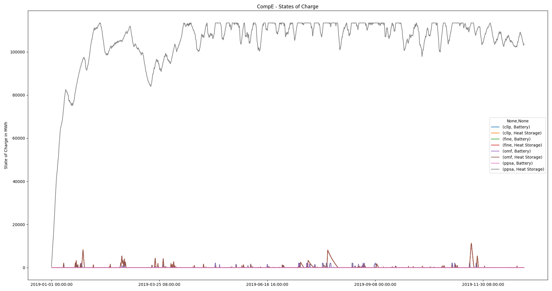
Comparing State-of-Charges (Checking Leftover ISD Hypotheses)

Visualizing the CompE MSC Storage SOCs for checking the hypotheses of large amounts of unused thermal energy.

Conclusion

Evaluating the findings from above, following conlusive can be drawn:

The tabular parameter comparison above shows, that all supported software tools, including PyPSA, are indeed able to model non-cyclic state-of-charge constraints for their storages, as is intended by Tessif in its CompE MSC.

Inspecting the state-of-charge results shows, that only PyPSA uses its 'Heat Storage' component to store large amounts of unneeded thermal energy.

Since all software tools successfully utilize a cyclic state-of-charge constraint, as shown by the plausibility check above, it seems reasonable, to assume that the observed use of the PyPSA 'Heat Storage Component', does not originate from the component itself, but is rather a side-effect of other factors. Based on the CHP component comparison above, it is seen as very likely, that the observed differences stem from the emission allocation issue resulting in an overall lower amount of detected emissions by PyPSA. Thus, resulting in the usage of the more cost efficient CHP components. Hence the same recommandation as above is made, with regards to reallocation and reoptimization of the Component Expansion MSC.

Storage Components and Emissions

Parameter Analysis

The table below lists the relavant part of the storage component’s tabular parameter comparison for Tessif and PyPSA

Parameter	Tessif	PyPSA
Component	Storage	StorageUnit
Identifier	Uid	name
Connecting Input(s)	input	bus
Connecting Output(s)	output
Installed Storage Capacity	capacity	max_hours * p_nom
Initial State of Charge	initial_soc	state_of_charge_initial
Final State of Charge	final_soc
Cyclic State of Charge	initial_soc = final_soc	cyclic_state_of_charge
Idle Positive Changes in State of Charge	idle_changes.positive	inflow
Idle Negative Changes in State of Charge	idle_changes.negative	standing_loss
Energy Flow Specific Charge Efficiencies	flow_efficiencies	efficiency_store
Energy Flow Specific Discharge Efficiencies	flow_efficiencies	efficiency_dispatch
Energy Flow Specific Flow Cost	flow_costs	marginal_cost
Energy Flow Specific Emissions	flow emissions

The Tabular comparison shows, that the PyPSA storage component does not have an inherent emission allocation parameter. As indicated in the CHP IRC Analysis, PyPSA uses seperate 'Carrier' objects to allocate emissions to (primary) energy carriers. Tessif utilizes them in creating an individual component specific 'Carrier' object, whith the respective emmisions allocated.

For the modified CompE MSC, Tessif allocates emissions to the 'Battery' as shown by the respective parameter analysis shown in the table below:

Parameter	Parameter Values
capacity	100
costs_for_being_active	0.0
expandable	{‘capacity’: True, ‘electricity’: True}
expansion_costs	{‘capacity’: 1630000, ‘electricity’: 0}
expansion_limits	{‘capacity’: MinMax(min=100, max=inf), ‘electricity’: MinMax(min=33, max=inf)}
final_soc
fixed_expansion_ratios	{‘electricity’: True}
flow_costs	{‘electricity’: 400}
flow_efficiencies	{‘electricity’: InOut(inflow=0.95, outflow=0.95)}
flow_emissions	{‘electricity’: 0.06}
flow_gradients	{‘electricity’: PositiveNegative(positive=inf, negative=inf)}
flow_rates	{‘electricity’: MinMax(min=0, max=33)}
gradient_costs	{‘electricity’: PositiveNegative(positive=0, negative=0)}
idle_changes	PositiveNegative(positive=0, negative=0.5)
initial_soc	0
initial_status	1
input	electricity
interfaces	frozenset({‘electricity’})
milp	{‘electricity’: False}
number_of_status_changes	OnOff(on=inf, off=inf)
output	electricity
status_changing_costs	OnOff(on=0.0, off=0.0)
status_inertia	OnOff(on=0, off=0)
timeseries
uid	Battery

This 'Battery' component specific carrier gets added, as shown by the respective PyPSA parameter analysis results, seen in the table below:

StorageUnit	carrier
Battery	Battery.carrier
Heat Storage

Further analysing the PyPSA allocated emissions shows, that the 'Battery' component gets the emission parameter succesfully allocated as listed in the table below:

Carrier	co2_emissions	color	nice_name	max_growth
Battery.carrier	0.06			inf
Solar Panel.carrier	0.05			inf
Onshore Wind Turbine.carrier	0.02			inf
Offshore Wind Turbine.carrier	0.02			inf
Hard Coal Supply.carrier	0.3440000000000001			inf
Biogas Supply.carrier	0.109375			inf
Combined Cycle PP.carrier	0.21			inf
Hard Coal PP.carrier	0.34400000000000003			inf
Lignite Power Plant.carrier	0.4			inf
Heat Plant.carrier	0.20700000000000002			inf
Power To Heat.carrier	0.000693			inf

Inspecting PyPSA's formulation on calculating the emissions as done by Reimer and Ammon shows that only the difference between final and initial state of charge are taken into account when calculating sotrage component related emisssions. Tessif however, intends the emissions to be allocated to the storage component outflow.

Plausibility Check

System-Model MSC:

• 'Demand' requires 10 energy units per time step over a total of four timesteps

• 'Initial Charge' provides 110 energy units at the first time step for zero cost units at zero emission, but none at the remaining time steps

• 'Battery' gets charged at the first time step with 100 energy units, has no outflow costs and no idle changes in its SOC.

• 'Battery' emitts 1 emission unit per energy unit flowing out of it

• Global emission constraint is set to 20 emission units

Expected outcome:

• Demand is met at the first timestep by the 'Initial Charge' component

• Demand is met at second and third time step by dischraging the 'Battery' component.

• At the last time step, global emission limit is reached due to the 'Battery' component discharging. Hence the 'Expensive' component meets the demand at the final timestep.

Observed outcome:

• Each of the software tools checked, with the exception of PyPSA, produce the expected outcome

• PyPSA however does not, and discharges the 'Battery' component at the third timestep to meet the demand, as shown in the upper table below. Leading to an overall emission of 30 emission units as interpreted by Tessif as seen in the lower table below.

• The results indicate, that PyPSA 'Storage Unit' components indeed calculate emissions based on SOC differences, in contrast to Tessif's outflow based calculation.

	cllp	cllp	fine	fine	omf	omf	ppsa	ppsa
Central Bus	Battery	Battery	Battery	Battery	Battery	Battery	Battery	Battery
2022-01-01 00:00:00	-0.0	100.0	-0.0	100.0	-0.0	100.0	-0.0	100.0
2022-01-01 01:00:00	-0.0	0.0	-10.0	0.0	-10.0	0.0	-10.0	0.0
2022-01-01 02:00:00	-10.0	0.0	-10.0	0.0	-10.0	0.0	-10.0	0.0
2022-01-01 03:00:00	-10.0	0.0	-0.0	0.0	-0.0	0.0	-10.0	0.0

Parameter	Results
emissions (sim)	30.0
costs (sim)	0.0
opex (ppcd)	0.0
capex (ppcd)	0.0

Conclusion

Summerizing the above investigations, following conlusive points can be made.

The PyPSA 'Battery' component emissions get succesfully allocated, as shown by the above Parameter Analysis and as obeservable in the emissions caused plot created during the preliminary result analysis.

Furthermore it could be shown, that PyPSA 'Storage' components do respect the emission allocation parameter. Emissions caused however, are calculated based on the difference between the final and initial state of charge, as indicated by the analysis of Reimer and Ammon and demonstrated by the Plausibility Check.

Since this discrepency can not easily be circumvented, by Tessif's current implementation, Reimer and Ammon investigated an additional modified CompE MSC in which no emissions were allocated to the storage components. Resulting in integrated global results, very close to each other (relative deviation less than one percent), including the emission results. Plausifying the findings of this root cause analysis.