Discussion/Overview
Generic Graph
The system model used for the LossLC combination can be seen below:
Optimization Results
The LossLC results are listed below. By convention, tessif uses
dynamic dimensioning to allow for different scales of amount of energy
transferred. The current conventions can be seen/adjusted via
tessif.frused.configurations and are as follows for the results below:
MW– for energy flows and installed power capacities
MWh– for amounts of energy and installed storage capacities
EUR– for costs
t_CO2– for emissions (tonns CO2 equivalent)
The LossLC results are generated using the skript from below and are as follows:
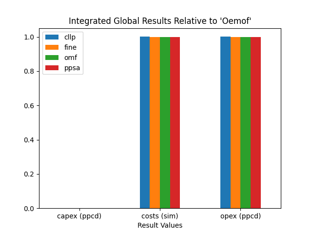
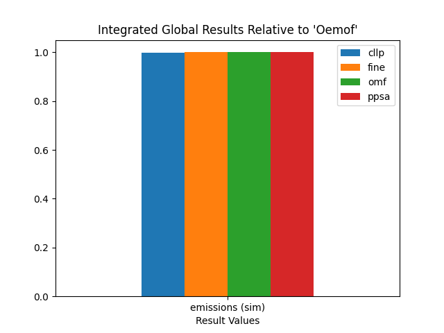
Integrated Global Results
IGR [€ or t_CO2] |
cllp |
fine |
omf |
ppsa |
capex (ppcd) |
0 |
0 |
0 |
0 |
costs (sim) |
202437193 |
202259102 |
202259102 |
202259102 |
emissions (sim) |
441567 |
443159 |
443159 |
443159 |
opex (ppcd) |
202437194 |
202259103 |
202259103 |
202259103 |
The Integrated Global Result bar plots are created using the code below.
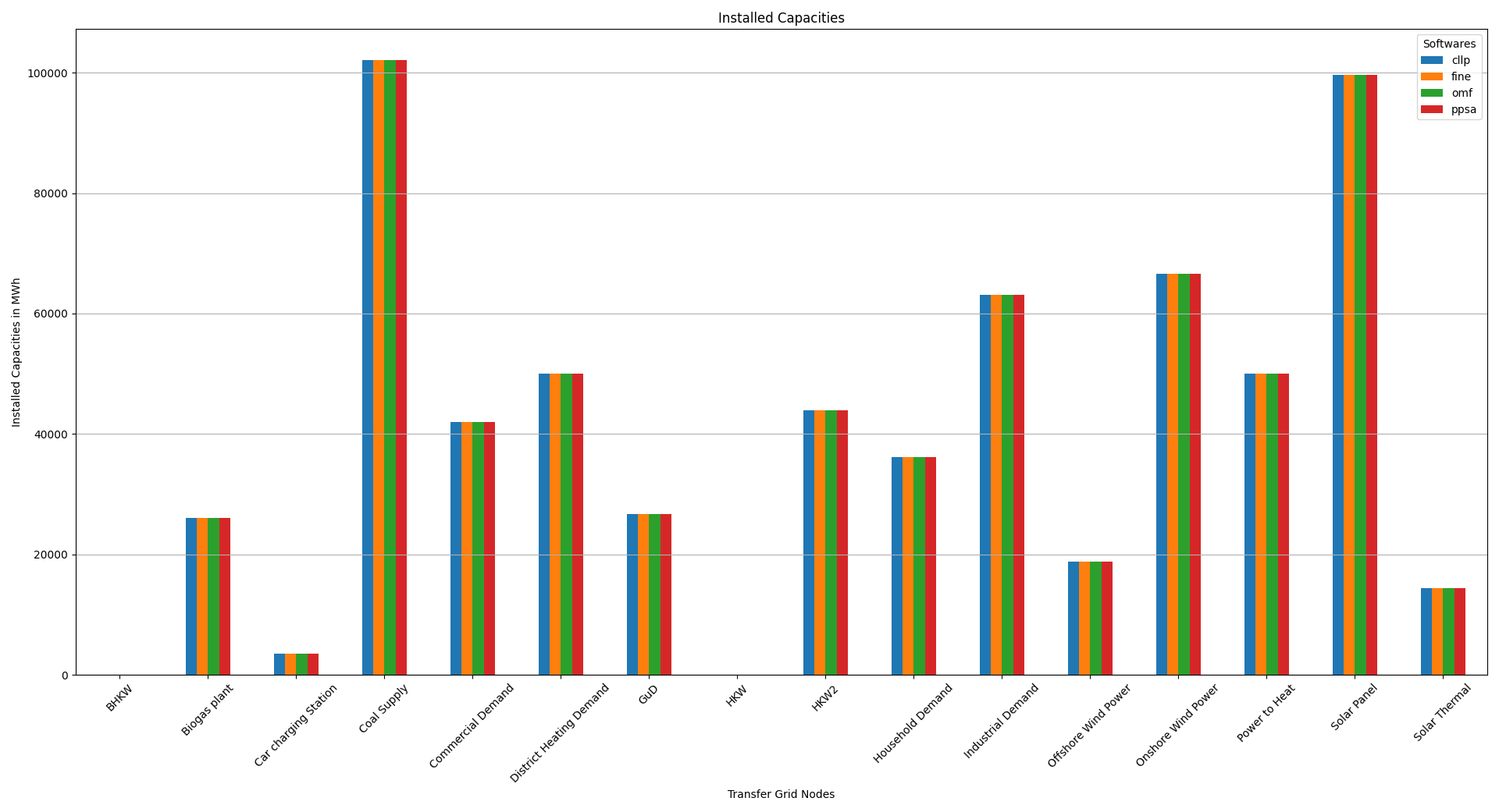
Installed Capacity
Capacity [MW or MWh] |
cllp |
fine |
omf |
ppsa |
BHKW |
[13513.696969697, 8576.0] |
[13513.697, 8576.0] |
[8576.0, 13513.69697] |
[13513.69697, 8576.0000001923] |
Biogas |
variable |
variable |
variable |
variable |
Biogas plant |
25987 |
25987 |
25987 |
25987 |
Car charging Station |
3473 |
3473 |
3473 |
3473 |
Coal Supply |
102123 |
102123 |
102123 |
102123 |
Coal Supply Line |
variable |
variable |
variable |
variable |
Commercial Demand |
41969 |
41969 |
41969 |
41969 |
District Heating |
variable |
variable |
variable |
variable |
District Heating Demand |
50000 |
50000 |
50000 |
50000 |
Gas Station |
45325 |
45325 |
45325 |
variable |
Gaspipeline |
variable |
variable |
variable |
variable |
GuD |
26742 |
26742 |
26742 |
26742 |
HKW |
[61273.96, 24509.584] |
[61273.998, 24509.599] |
[61273.96, 24509.6] |
[61273.96, 24509.584] |
HKW2 |
43913 |
43913 |
43913 |
43913 |
High Voltage Grid |
variable |
variable |
variable |
variable |
High Voltage Transfer Grid |
variable |
0 |
variable |
72141 |
Household Demand |
36177 |
36177 |
36177 |
36177 |
Industrial Demand |
63093 |
63093 |
63093 |
63093 |
Low Voltage Grid |
variable |
variable |
variable |
variable |
Low Voltage Transfer Grid |
variable |
54703 |
variable |
54703 |
Medium Voltage Grid |
variable |
variable |
variable |
variable |
Offshore Wind Power |
18760 |
18760 |
18760 |
18760 |
Onshore Wind Power |
66599 |
66599 |
66599 |
66599 |
Power to Heat |
50000 |
50000 |
50000 |
50000 |
Solar Panel |
99605 |
99605 |
99605 |
99605 |
Solar Thermal |
14343 |
14343 |
14343 |
14343 |
Medium Voltage Grid Summed Loads
Load-Medium Voltage Grid [MW] |
cllp |
fine |
omf |
ppsa |
Car charging Station |
37026 |
37026 |
37026 |
37026 |
High Voltage Transfer Grid |
-867448 |
-871089 |
-871089 |
-871089 |
High Voltage Transfer Grid |
0 |
0 |
0 |
0 |
Industrial Demand |
1229008 |
1229008 |
1229008 |
1229008 |
Low Voltage Transfer Grid |
-111125 |
-111125 |
-111125 |
-111125 |
Low Voltage Transfer Grid |
640388 |
644028 |
644028 |
644028 |
Onshore Wind Power |
-1099866 |
-1099866 |
-1099866 |
-1099866 |
Power to Heat |
172017 |
172017 |
172017 |
172017 |
Computational Ressources Used
The computational results are generated using the respective estimation scripts as well as the subsequent plotting scripts.
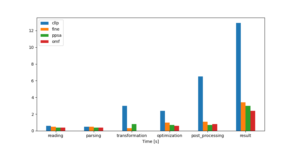
Timings Results
Time [s] |
cllp |
fine |
ppsa |
omf |
reading |
0.6 |
0.5 |
0.4 |
0.4 |
parsing |
0.5 |
0.5 |
0.4 |
0.4 |
transformation |
3.0 |
0.3 |
0.8 |
0.0 |
optimization |
2.4 |
1.0 |
0.7 |
0.6 |
post_processing |
6.5 |
1.1 |
0.7 |
0.8 |
result |
12.9 |
3.4 |
3.0 |
2.4 |
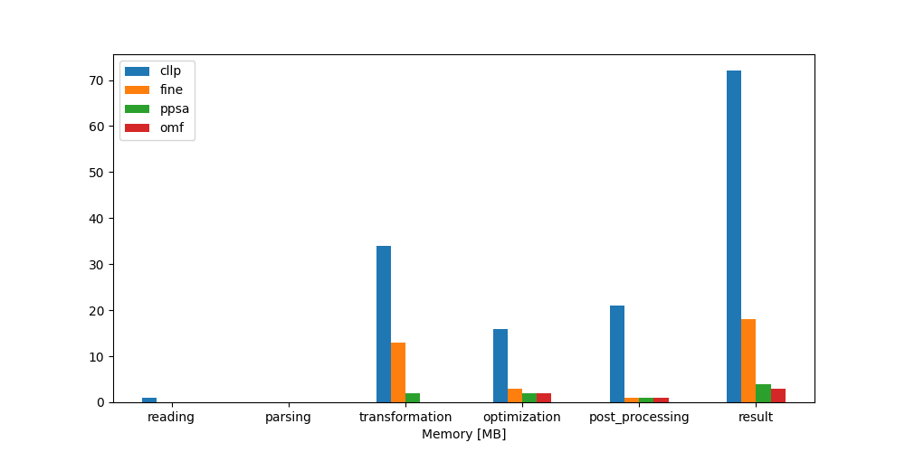
Memory Results
Memory [MB] |
cllp |
fine |
ppsa |
omf |
reading |
1.0 |
0.0 |
0.0 |
0.0 |
parsing |
0.0 |
0.0 |
0.0 |
0.0 |
transformation |
34.0 |
13.0 |
2.0 |
0.0 |
optimization |
16.0 |
3.0 |
2.0 |
2.0 |
post_processing |
21.0 |
1.0 |
1.0 |
1.0 |
result |
72.0 |
18.0 |
4.0 |
3.0 |
Key Conclusions
The Key Goal could be served in the sense of developing a reference supply system model in conjunction with one of the two relevant and contemporary scenario formulations (
commitment-problem) to test out the modelling softwaresCalliope,Fine,OemofandPypsa.None of the 4 aims formulated, with regards to gird focused model behaviour, are specifically addressed with this
'Lossless Commitment'model scenario combination. It however lays the foundation for the Transformer Commitment/Expansion which directly address all of these aims.Even on a relatively complex model-scenario-combination modelling ideal grid behaviours it could be shown that the optimal solutions found, using the softwares
Calliope,Fine,OemofandPypsathrough tessif, deviate by less than1%relative to each other.