system_loads

bars	Draw a sophisticated bar plot for visualizing energy system load data.
bars_from_es	Draw sytem model energy "generation" as advanced bar plot.

Powerful bar drawing utility based on matplotlib.pyplot.bar().

While it is designed to quickly draw arbitrarily complex bar charts representing energy system loads, it can be used as standalone drawing utility for really just any bar chart.

Algorithm is build on a triple nested list engine which is able to visualize plot data grouped as [category [subcategory [data]]]

Default coloring uses tessif.frused.themes.colors and cmaps.

tessif.visualize.system_loads.bars(loads, index=[], category_labels=[], category_colors=[], category_hatches=[], labels=[], colors=[], hatches=[], dticks=1, offset=0, fmt='%a. %m-%d', ylabel='Power in MWh', **kwargs)

Draw a sophisticated bar plot for visualizing energy system load data.

Works on a simple yet powerfull nested list engine. Able to automatically draw a simple bar chart or a full fledged energy system load analysis split by major and minor categorization options. Minor categorization uses triple nested lists, whereas major parameters are represented as double layer nested lists. See parameters for details. Calls matplotlib.pyplot.bar().

Parameters:

• loads (Iterable) –

  Iterable of numbers i.e. list, pandas.Series or pandas.DataFrame etc. To be plotted data will be transformed into a triple nested list as:

  [  # Category Level
      [  # Subcategory Level
          [  # Data Level
          ]
      ]
  ]
  

  • Upper most level:

    [Sector 1, …, Sector N]

  • In between:

    [Subcategory 1, …, Subcategory N] for each category

  • Lowest level:

    [Load at timestep 1, …. load at timestep N] for each subcategory

  Any nesting depth <= 3 can be handled and will be interpreted as stated above

• index (Iterable, default = []) –

  Iterable of integers or entries on which strftime can be called.

  Use it to:

  • plot data over unequidistant indices (equidistant as in range(0, len(laod), dticks) e.g [3, 8, 20]

  • Print date/time/date/time strings as ticklabels, e.g: list(pd.DataFrame.index)

• category_labels (Iterable, default=[]) –

  Iterable container of strings used to label category level entries. i.e.: ['Power', 'Heat', 'Mobility']

  Beware:

  • len(category_labels) !>= number of categories

  • Use None to not draw any major labels.

  • Use default to tag the n-th category by ‘Category N’

• category_colors (Iterable, default=[]) –

  Iterable container of color strings used to color major categories when drawing the major category plot. i.e.: ['yellow', 'red' 'blue']

  Beware:

  • len(category_colors) !>= number of categories

  • Use None to use matplotlib’s default coloring cycle.

  • Use [] (default) to invoke the tessif.frused.themes.colors coloring.

• category_hatches (Iterable, default=[]) –

  iterable container of hatch strings used to hatch major categories when drawing the major category plot. i.e.: ['/', '\ ' '+']

  Supported patterns: {'/', '\\', '|', '-', '+', 'x', 'o', 'O', '.', '*'}

  Beware:

  • len(category_hatches) !>= number of categories

  • Use None to not hatch at all

  • Use [] (default) to invoke the tessif.frused.themes.hatches hatching

• labels (Iterable, default=[]) –

  iterable container of strings used to tag subcategory level entries. i.e : [['PV', 'Wind'], ['Gas', 'ST'], ['Diesel', 'Petrol']] Nest entries intuitively the way the loads are nested.

  Beware:

  • len(labels) !>= number of categories

  • len(nested_labels) !>= number of respective subcategory entries

  • Use None to not tag any subcategory level entries

  • Use [] (default) to tag the n-th subcategory entry by ‘Subcategory N’

• colors (Iterable, default=[]) –

  iterable container of strings used to color subcategory level entries. i.e: [['yellow' , '#123456'], ['red', 'crimson'], ['pink', 'black']] Nest entries intuitively the way the loads are nested.

  Beware:

  • len(colors) !>= number of categories

  • len(nested_colors) !>= number of respective subcategories

  • Use None to use matplotlib’s default coloring cycle.

  • Use [] (default) to invoke the tessif.frused.themes.cmaps coloring.

• hatches (Iterable, default=[]) –

  Iterable container of strings used to hatch subcategory level entries. i.e: [['/', '\ '], ['|', '-'], ['o', '*']]

  Supported patterns: {'/', '\\', '|', '-', '+', 'x', 'o', 'O', '.', '*'}

  Beware:

  • len(hatches) !>= number of categories

  • len(nested_hatches) !>= number of respective subcategories

  • Use None to not hatch any subcategory level entry

  • Use [] (default) to invoke the tessif.frused.themes.hmaps hatching.

• dticks (positive scalar, optional, default = 1) –

  X axis tick distance in number of load entries.

  i.e dticks=12 with an hourly resolution of load level entries results in a tick every 12 hours.

• offset (positive scalar, optional, default = 0) –

  Amount of load entries the tick labels are moved.

  i.e offset=10 with an hourly resolution of load level entries moves all tick labels by 10 hours to the right.

• fmt (str, optional) –

  Date formatting string used to format and display tick labels if an index of type date/time/datetime was provided.

  i.e.: fmt='%a. %m-%d' of date(1, 1, 1) results in ‘Mon. 01-01’

  See strftime() and strptime() Behavior for more details.

• kwargs – kwargs are passed to matplotlib.pyplot.bar()

Notes

The first load entry is drawn on top. This behavior was chosen cause the author thinks of it as the most intuitive way of bar plotting. To archieve that the algorithm reverses all iterables. Keep that in mind when providing iterables too long for one of the optional parameters cause this will lead to the first entries beeing dropped, not the last!

Examples

>>> import matplotlib.pyplot as plt
>>> from tessif.visualize import system_loads

Creating the most simple bar plot examplifying:

• Using plot() as simple bar plot wrapper

• None usage to supress features

• Omitting the outer iterable on the optional parameters

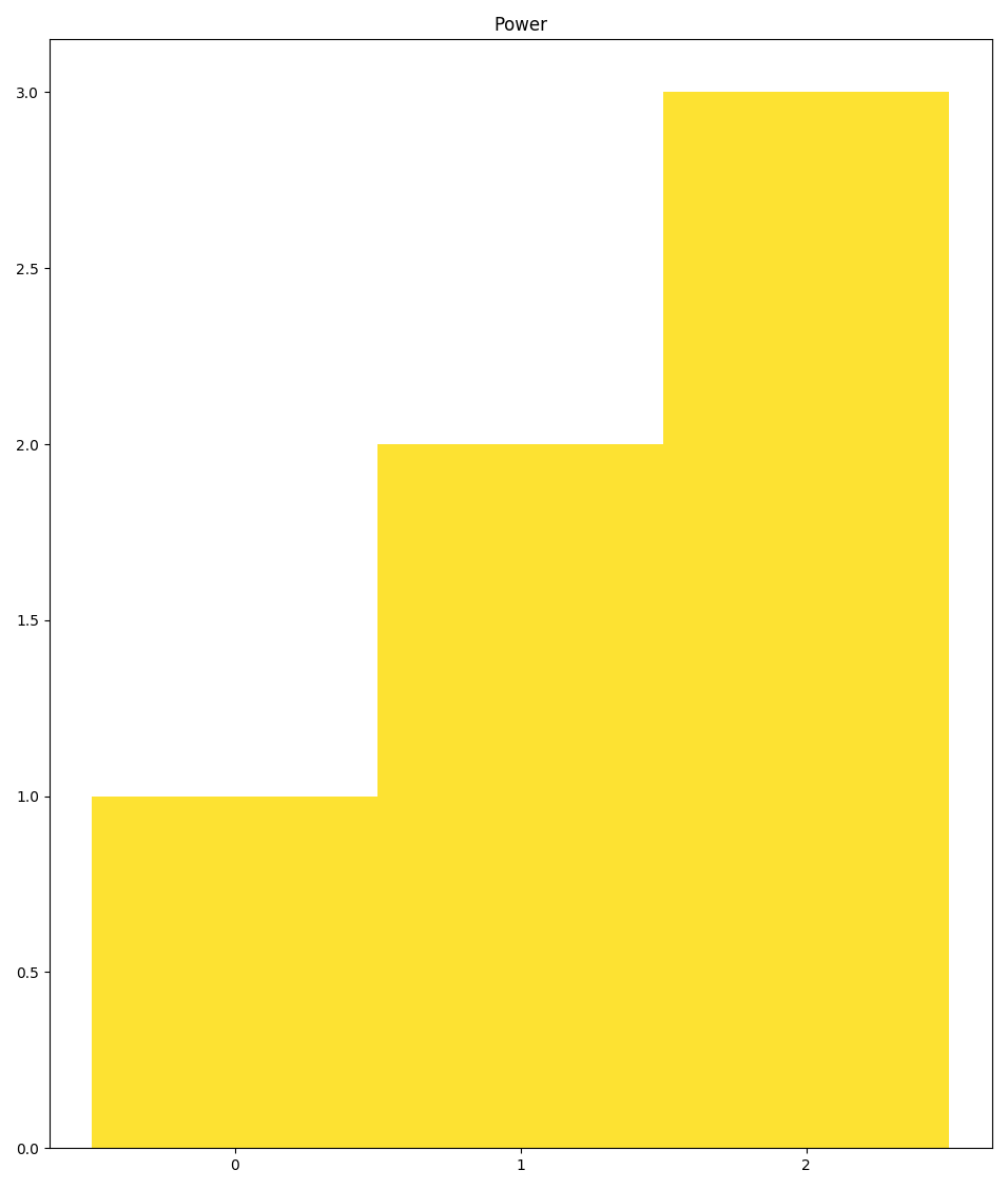
>>> axes = system_loads.bars(
...     loads=[1,2,3],  # one load series
...     labels=None,   # None to suppress feature
...     category_labels='Power',  # Omitting outer iterable
...     hatches=None)
>>> # axes.figure.show() # commented out for doctesting

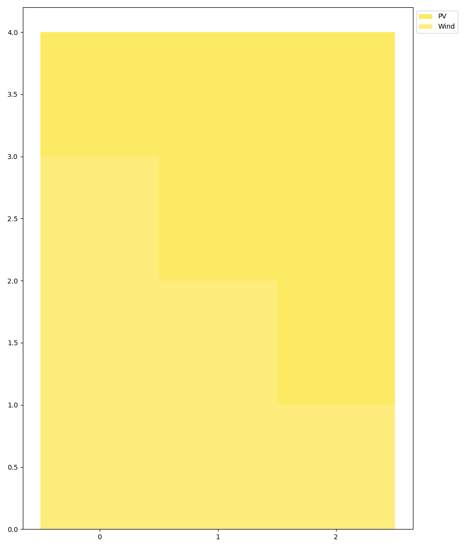
Creating a bar plot with 2 subcategories of the same category:

>>> axes = system_loads.bars(
...     loads=[[1, 2, 3], [3, 2, 1]],  # 1 cat of 2 subcats of 3 loads each
...     labels=['PV', 'Wind'],   # 2 subcats, 2 labels
...     category_labels=None,  # Use None to suppress features
...     hatches=None)
>>> # axes.figure.show() # commented out for doctesting

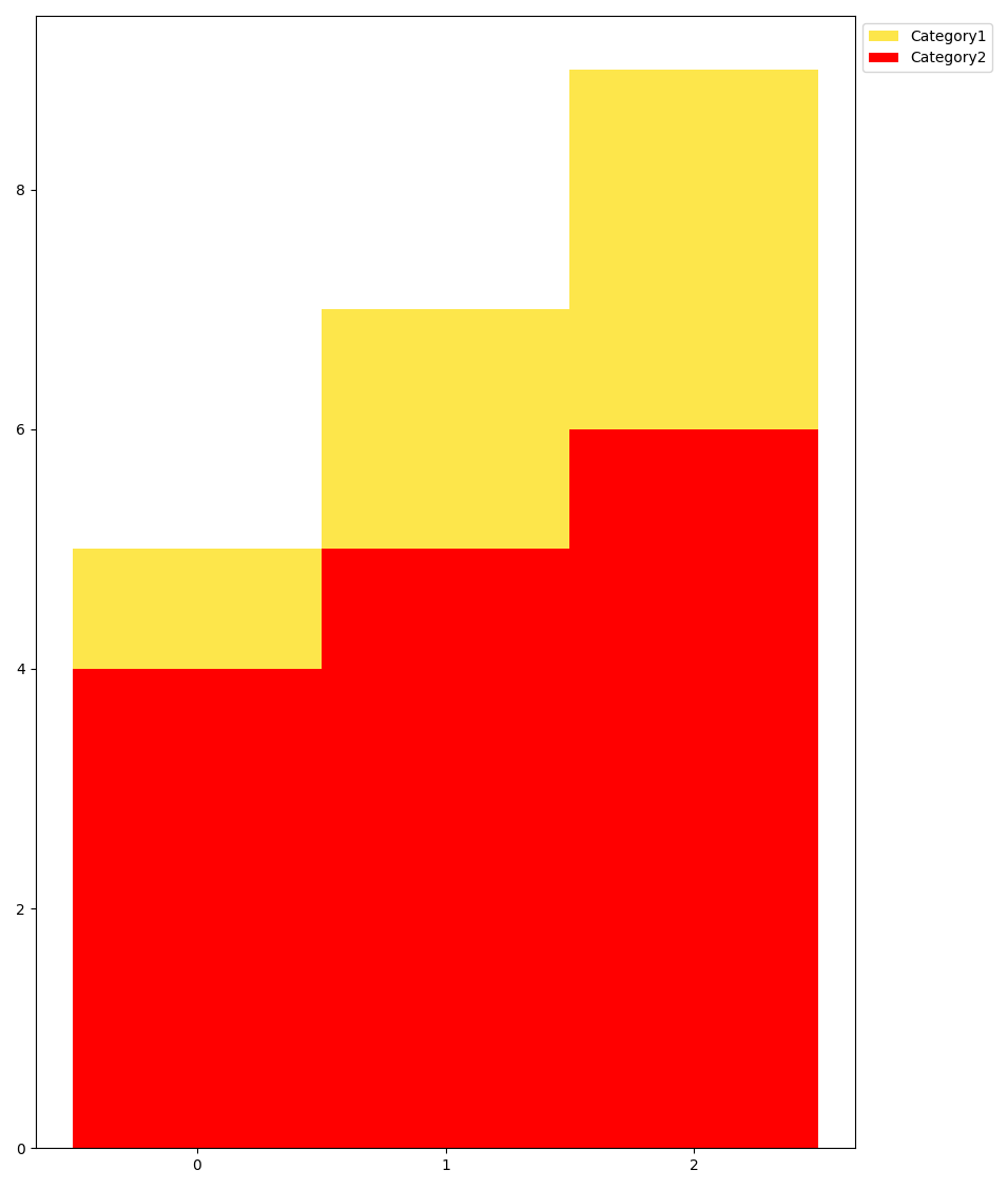
Creating a bar plot with 2 categories of 1 subcategory each:

>>> axes = system_loads.bars(
...     loads=[[[1, 2, 3]], [[4, 5, 6]]],  # 2 cats 1 subcat each
...     # Beware of appropriate nesting when not using all levels:
...     labels=[['Power'], ['Heat']],
...     # Use default (empty list) to tag loads by 'Category N'
...     category_labels=[],
...     hatches=None)
>>> # axes.figure.show() # commented out for doctesting

Creating an energy system load analysis bar plot with 2 categoriess with 3/2 subcategories:

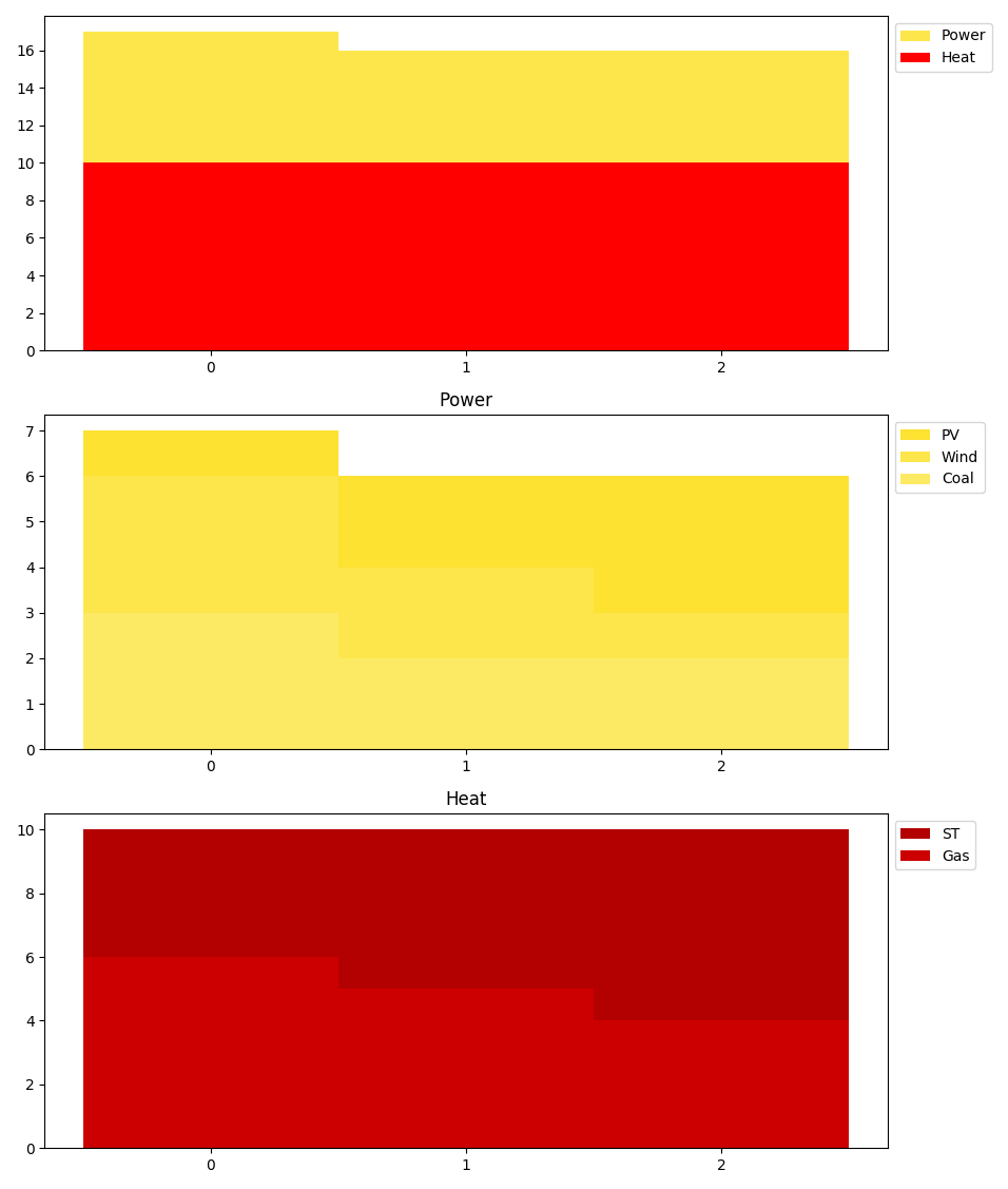
>>> axes = system_loads.bars(
...     loads=[[[1, 2, 3], [3, 2, 1], [3, 2, 2]],
...           [[4, 5, 6], [6, 5, 4]]],
...     # labels are nested intuitively
...     labels=[['PV', 'Wind', 'Coal'], ['ST', 'Gas', ]],
...     # All kinds of iterables are supported:
...     category_labels=('Power', 'Heat'),
...     hatches=None)
>>> # axes.figure.show() # commented out for doctesting

Creating an energy system load analysis bar plot - Design Case:

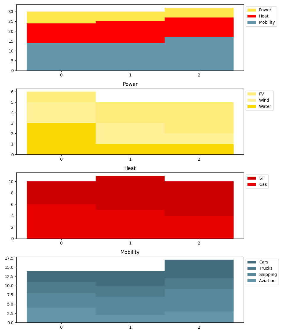
>>> axes = system_loads.bars(
...     # 3 cats, 3/2/4 subs
...     loads=[[[1, 2, 3], [2, 2, 1], [3, 1, 1]],
...            [[4, 6, 6], [6, 5, 4]],
...            [[3, 4, 5], [3, 3, 3], [4, 5, 6], [4, 2, 3]]],
...     # Varying subcat lengths
...     labels=[['PV', 'Wind', 'Water'], ['ST', 'Gas'],
...             ['Cars', 'Trucks', 'Shipping', 'Aviation']],
...     # All kinds of iterables are supported:
...     category_labels=('Power', 'Heat', 'Mobility'),
...     hatches=None)
>>> # axes.figure.show() # commented out for doctesting

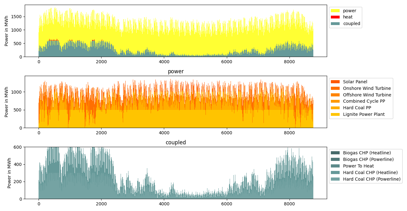
tessif.visualize.system_loads.bars_from_es(optimized_es, ignore=None, drop_zeros=True, **kwargs)

Draw sytem model energy “generation” as advanced bar plot.

Convenience wrapper for bars(). Load results are automatically sorted by sector to draw a stacked bar plot for each sector in conjunction with an overall stacked bar plot of the entire model-scenario-combination results.

Parameters:

• optimized_es – Optimized energy supply system model scenario combination. Usually returned by one of the respective tessif.simulate functionalities.

• ignore (Container, None, default=None) – Container of node uid representations to not be included

• drop_zeros (bool, default=True) – If True all zero loads will be dropped. This can however lead unsuccesfull plotting. In this case zero columns need to be kept and nodes ignored manually using ignore

• kwargs – Key word arguments are passed to bars()

Returns:

Matplotlib axes object holding the plotted figure elements.

Return type:

matplotlib.axes

Examples

When using bars_from_es() usually two usecases occur.

1. Dropping all-zero entries because each sector has at least one not-all-zeros-load associated. But there are still some commodity sources present which need to be ignored manually for a sensible plot:

   >>> import tessif.examples.data.tsf.py_hard as hardcoded_tsf_examples
   >>> hh_msc = hardcoded_tsf_examples.create_hhes()
   

   >>> component_msc = hardcoded_tsf_examples.create_component_es(periods=50)
   

   >>> import tessif.transform.es2es.omf as tsf2omf  # nopep8
   >>> oemof_hh_msc = tsf2omf.transform(hh_msc)
   >>> oemof_comp_msc = tsf2omf.transform(component_msc)
   

   >>> import tessif.simulate  # nopep8
   >>> optimized_oemof_hh_msc = tessif.simulate.omf_from_es(oemof_hh_msc)
   >>> optimized_oemof_comp_msc = tessif.simulate.omf_from_es(oemof_comp_msc)
   

   >>> from tessif.visualize import system_loads  # nopep8
   >>> axes = system_loads.bars_from_es(
   ...     optimized_oemof_hh_msc,
   ...     drop_zeros=True,
   ...     ignore=[
   ...         "coal supply",
   ...         "biomass supply",
   ...     ],
   ... )
   >>> # axes.figure.show() # commented out for doctesting
   

   For the image shown the model-scenario-combination was optimized using periods=8760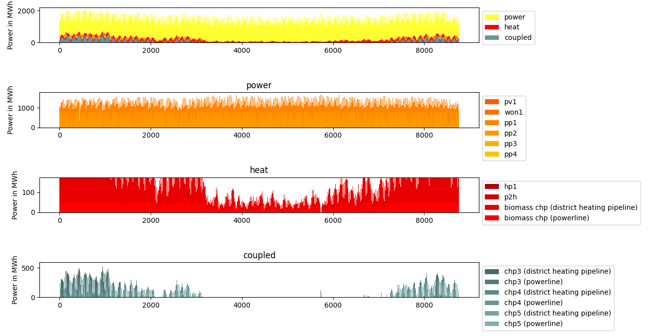

   

2. Not dropping all-zero entries, because at least one sector consists of only all-zeros-loads, is required, to enable plotting. In addition some commodity sources are ignored manually to draw a sensible plot:

   >>> import tessif.examples.data.tsf.py_hard as hardcoded_tsf_examples
   >>> component_msc = hardcoded_tsf_examples.create_component_es(periods=25)
   

   >>> import tessif.transform.es2es.omf as tsf2omf  # nopep8
   >>> oemof_comp_msc = tsf2omf.transform(component_msc)
   

   >>> import tessif.simulate  # nopep8
   >>> optimized_oemof_comp_msc = tessif.simulate.omf_from_es(
   ...     oemof_comp_msc)
   

   >>> from tessif.visualize import system_loads  # nopep8
   >>> axes = system_loads.bars_from_es(
   ...     optimized_oemof_hh_msc,
   ...     drop_zeros=False,
   ...     ignore=[
   ...          "Gas Station",
   ...          "Hard Coal Supply",
   ...          "Lignite Supply",
   ...          "Biogas Supply",
   ...     ],
   ... )
   >>> # axes.figure.show() # commented out for doctesting
   

   For the image shown the model-scenario-combination was optimized using periods=8760