Transshipment Problem Example (Brief)
This example briefly illustrates the auto comparative features of the
analyze module. For a more detailed example please refer to
the Fully Parameterized Working Example (Detailed).
Initial code to do the comparison
>>> # change spellings_logging_level to debug to declutter output
>>> import tessif.frused.configurations as configurations
>>> configurations.spellings_logging_level = 'debug'
>>> # Import hardcoded tessif energy system using the example hub:
>>> import tessif.examples.data.tsf.py_hard as tsf_examples
>>> # Choose the underlying energy system
>>> tsf_es = tsf_examples.create_connected_es()
>>> # write it to disk, so the comparatier can read it out
>>> import os
>>> from tessif.frused.paths import write_dir
>>> #
>>> output_msg = tsf_es.to_hdf5(
...     directory=os.path.join(write_dir, 'tsf'),
...     filename='transshipment_comparison.hdf5',
... )
>>> # let the comparatier to the auto comparison:
>>> import tessif.analyze, tessif.parse
>>> #
>>> comparatier = tessif.analyze.Comparatier(
...     path=os.path.join(write_dir, 'tsf', 'transshipment_comparison.hdf5'),
...     parser=tessif.parse.hdf5,
...     models=('oemof', 'pypsa', 'fine', 'calliope'),
... )
Code accessing the results
Following section provides examples on how to use the
Comparatier interface to access the
auto generated comparison results.
Models
>>> # show the models compared:
>>> for model in sorted(comparatier.models):
...     print(model)
cllp
fine
omf
ppsa
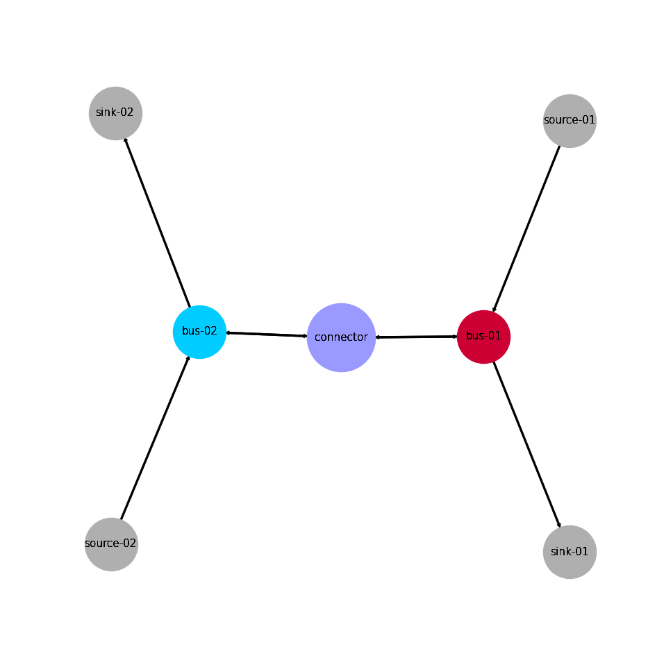
Energy System Graph
>>> import matplotlib.pyplot as plt
>>> import tessif.visualize.nxgrph as nxv
>>> grph = comparatier.graph
>>> drawing_data = nxv.draw_graph(
...     grph,
...     node_color={
...         'connector': '#9999ff',
...         'bus-01': '#cc0033',
...         'bus-02': '#00ccff',
...     },
...     node_size={'connector': 5000},
... )
>>> # plt.show()  # commented out for simpler doctesting
Comparative Model Results
Following sections show how to utilize to built-in
ComparativeResultier to access results conveniently
among models.
Load Results
>>> print(comparatier.comparative_results.loads['connector'])
                         cllp                           fine                            omf                        ppsa
connector              bus-01 bus-02 bus-01 bus-02    bus-01 bus-02 bus-01 bus-02    bus-01 bus-02 bus-01 bus-02 bus-01 bus-02 bus-01 bus-02
1990-07-13 00:00:00 -5.555556  -0.00    0.0    5.0 -5.555556  -0.00    0.0    5.0 -5.555556  -0.00    0.0    5.0   -5.0   -0.0    0.0    5.0
1990-07-13 01:00:00 -0.000000  -6.25    5.0    0.0 -0.000000  -6.25    5.0    0.0 -0.000000  -6.25    5.0    0.0   -0.0  -10.0   10.0    0.0
1990-07-13 02:00:00 -0.000000  -0.00    0.0    0.0 -0.000000  -0.00    0.0    0.0 -0.000000  -0.00    0.0    0.0   -0.0   -0.0    0.0    0.0
Note
Note how connector flows vary between models. This is due to the fact, that
pypsa connectors
do not handle bidirectional flows well with efficiencies other than 1.0, whereas
oemof connectors do.
Hence tessif sets bidirectional tessif connector efficiencies to 1.0 when
transforming into pypsa connectors.
>>> print(comparatier.comparative_results.loads['bus-01'])
                         cllp                                   fine                                    omf                                   ppsa
bus-01              connector  source-01 connector sink-01 connector  source-01 connector sink-01 connector  source-01 connector sink-01 connector source-01 connector sink-01
1990-07-13 00:00:00      -0.0  -5.555556  5.555556     0.0      -0.0  -5.555556  5.555556     0.0      -0.0  -5.555556  5.555556     0.0      -0.0      -5.0       5.0     0.0
1990-07-13 01:00:00      -5.0 -10.000000  0.000000    15.0      -5.0 -10.000000  0.000000    15.0      -5.0 -10.000000  0.000000    15.0     -10.0      -5.0       0.0    15.0
1990-07-13 02:00:00      -0.0 -10.000000  0.000000    10.0      -0.0 -10.000000  0.000000    10.0      -0.0 -10.000000  0.000000    10.0      -0.0     -10.0       0.0    10.0
>>> print(comparatier.comparative_results.loads['bus-02'])
                         cllp                                  fine                                   omf                                  ppsa
bus-02              connector source-02 connector sink-02 connector source-02 connector sink-02 connector source-02 connector sink-02 connector source-02 connector sink-02
1990-07-13 00:00:00      -5.0    -10.00      0.00    15.0      -5.0    -10.00      0.00    15.0      -5.0    -10.00      0.00    15.0      -5.0     -10.0       0.0    15.0
1990-07-13 01:00:00      -0.0     -6.25      6.25     0.0      -0.0     -6.25      6.25     0.0      -0.0     -6.25      6.25     0.0      -0.0     -10.0      10.0     0.0
1990-07-13 02:00:00      -0.0    -10.00      0.00    10.0      -0.0    -10.00      0.00    10.0      -0.0    -10.00      0.00    10.0      -0.0     -10.0       0.0    10.0
Flow Cost Results
Connectors related flows:
>>> print(comparatier.comparative_results.costs[('connector', 'bus-01')])
cllp    0.0
fine    0.0
omf     0.0
ppsa    0.0
Name: (connector, bus-01), dtype: float64
>>> print(comparatier.comparative_results.costs[('bus-01', 'connector')])
cllp    0.0
fine    0.0
omf     0.0
ppsa    0.0
Name: (bus-01, connector), dtype: float64
>>> print(comparatier.comparative_results.costs[('connector', 'bus-02')])
cllp    0.0
fine    0.0
omf     0.0
ppsa    0.0
Name: (connector, bus-02), dtype: float64
>>> print(comparatier.comparative_results.costs[('bus-02', 'connector')])
cllp    0.0
fine    0.0
omf     0.0
ppsa    0.0
Name: (bus-02, connector), dtype: float64
Source related flows:
>>> print(comparatier.comparative_results.costs[('source-01', 'bus-01')])
cllp    1.0
fine    1.0
omf     1.0
ppsa    1.0
Name: (source-01, bus-01), dtype: float64
>>> print(comparatier.comparative_results.costs[('source-02', 'bus-02')])
cllp    1.0
fine    1.0
omf     1.0
ppsa    1.0
Name: (source-02, bus-02), dtype: float64
Flow Emission Results
Connectors related flows:
>>> print(comparatier.comparative_results.emissions[('connector', 'bus-01')])
cllp    0.0
fine    0.0
omf     0.0
ppsa    0.0
Name: (connector, bus-01), dtype: float64
>>> print(comparatier.comparative_results.emissions[('bus-01', 'connector')])
cllp    0.0
fine    0.0
omf     0.0
ppsa    0.0
Name: (bus-01, connector), dtype: float64
>>> print(comparatier.comparative_results.emissions[('connector', 'bus-02')])
cllp    0.0
fine    0.0
omf     0.0
ppsa    0.0
Name: (connector, bus-02), dtype: float64
>>> print(comparatier.comparative_results.emissions[('bus-02', 'connector')])
cllp    0.0
fine    0.0
omf     0.0
ppsa    0.0
Name: (bus-02, connector), dtype: float64
Source related flows:
>>> print(comparatier.comparative_results.emissions[('source-01', 'bus-01')])
cllp    0.8
fine    0.8
omf     0.8
ppsa    0.8
Name: (source-01, bus-01), dtype: float64
>>> print(comparatier.comparative_results.emissions[('source-02', 'bus-02')])
cllp    1.2
fine    1.2
omf     1.2
ppsa    1.2
Name: (source-02, bus-02), dtype: float64
Integrated Global Results (IGR)
Following section demonstrate how to access the
integrated global results of the models compared.
>>> # show the integrated global results of the storage example:
>>> comparatier.integrated_global_results.drop(
...     ['time (s)', 'memory (MB)'], axis='index')
                 cllp  fine   omf  ppsa
emissions (sim)  52.0  52.0  52.0  52.0
costs (sim)      52.0  52.0  52.0  50.0
opex (ppcd)      52.0  52.0  52.0  50.0
capex (ppcd)      0.0   0.0   0.0   0.0
Memory and timing results are dropped because they vary slightly between runs. The original results look something like:
comparatier.integrated_global_results

                 cllp  fine   omf  ppsa
emissions (sim)  52.0  52.0  52.0  52.0
costs (sim)      52.0  52.0  52.0  50.0
opex (ppcd)      52.0  52.0  52.0  50.0
capex (ppcd)      0.0   0.0   0.0   0.0
time (s)          0.6   0.7   0.5   1.0
memory (MB)       0.9   1.1   0.5   1.4