Quick Start

Following sections provide a - little talk, much code - introduction to tessif. Everything should be copy-pastable and work out of the box, given your installation of tessif was successful.

Transform es to oemof and pypsa and simulate it

In this example a minimal energy system is created in tessif, then transformed into both an oemof and a pypsa energy system and then each gets simulated.

1. Create the tessif energy system. Use the create_mwe() function from tessif’s example hub to get one of the hardcoded example energy systems:

   import tessif.examples.data.tsf.py_hard as tsf_examples
   tsf_es = tsf_examples.create_mwe()
   

Hint

Access the nodes of the energy system by iterating over them:

for node in tsf_es.nodes:
    print(node.uid)

2. Transform the tessif energy system into oemof and pypsa energy systems:

   import tessif.transform.es2es.omf as tsf2omf
   import tessif.transform.es2es.ppsa as tsf2pypsa
   oemof_es = tsf2omf.transform(tsf_es)
   pypsa_es = tsf2pypsa.transform(tsf_es)
   

3. Optimize the energy systems using tessif.simulate which is a wrapper for the simulation calls of the supported models (more info here):

   import tessif.simulate
   optimized_oemof_es = tessif.simulate.omf_from_es(oemof_es)
   optimized_pypsa_es = tessif.simulate.ppsa_from_es(pypsa_es)
   

4. Show some results with the help of tessif’s post processing utilities. In this example the loads of a specific node are shown.

   import tessif.transform.es2mapping.omf as post_process_oemof
   import tessif.transform.es2mapping.ppsa as post_process_pypsa
   oemof_load_results = post_process_oemof.LoadResultier(optimized_oemof_es)
   pypsa_load_results = post_process_pypsa.LoadResultier(optimized_pypsa_es)
   print(oemof_load_results.node_load['Powerline'])
   print(pypsa_load_results.node_load['Powerline'])
   

Automatically compare es optimized with different models

In this example a minimal energy system is created in tessif, then Comparatier is used to transform it into different models and perform automated comparisons between them, then ComparativeResultier is used to show some of the results.

1. Change spellings_logging_level to ‘debug’ to declutter the output:

   import tessif.frused.configurations as configurations
   configurations.spellings_logging_level = 'debug'
   

2. Create the tessif energy system and write it to disk. Use the create_mwe() function from tessif’s example hub to get one of the hardcoded example energy systems:

   import os
   import tessif.examples.data.tsf.py_hard as tsf_examples
   from tessif.frused.paths import write_dir
   tsf_es = tsf_examples.create_fpwe()
   output_msg = tsf_es.to_hdf5(
       directory=os.path.join(write_dir, 'tsf'),
       filename='fpwe_quick.hdf5',
   )
   

3. Let the Comparatier do the auto comparison:

   import tessif.analyze
   import tessif.parse
   comparatier = tessif.analyze.Comparatier(
       path=os.path.join(write_dir, 'tsf', 'fpwe_quick.hdf5'),
       parser=tessif.parse.hdf5,
       models=('oemof', 'pypsa'),
   )
   

4. Access the results. What follows are some examples for the kinds of results that are available. More can be found here.

   Print the flow emissions of a specific edge:

   print(comparatier.comparative_results.emissions[('Generator', 'Powerline')])
   

   returns:

   omf     10.000000
   ppsa    17.142857
   Name: (Generator, Powerline), dtype: float64
   

   Print the computation time used by each model:

   import pprint
   for model, timing_results in comparatier.timing_results.items():
       print(model)
       print(79*'-')
       pprint.pprint(timing_results)
       print(79*'-')
   

   returns:

   omf
   -------------------------------------------------------------------------------
   {'parsing': 2,
    'post_processing': 5,
    'reading': 1,
    'simulation': 4,
    'transformation': 3}
   -------------------------------------------------------------------------------
   ppsa
   -------------------------------------------------------------------------------
   {'parsing': 2,
    'post_processing': 5,
    'reading': 1,
    'simulation': 4,
    'transformation': 3}
   -------------------------------------------------------------------------------
   

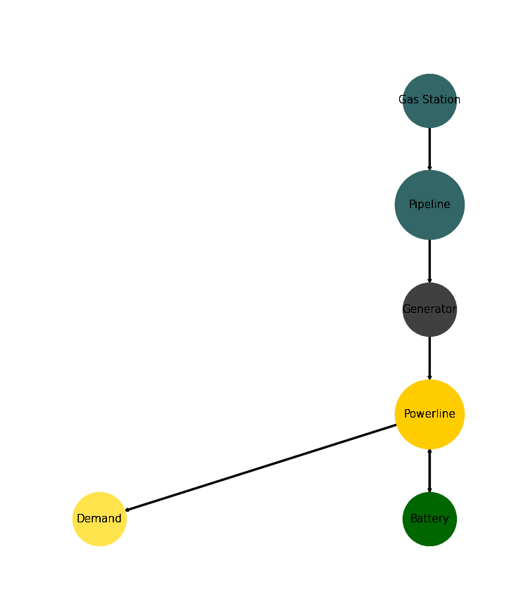
Visualize an energy system

In this example a minimal energy system is created in tessif, then transformed into a networkx.DiGraph object and then visualized using the nxgrph module's function draw_graph(). More info on visualizing energy systems can be found here.

1. Create the tessif energy system. Use the create_mwe() function from tessif’s example hub to get one of the hardcoded example energy systems:

   import tessif.examples.data.tsf.py_hard as tsf_examples
   es = tsf_examples.create_mwe()
   

2. Use the energy system's method to_nxgrph() to create a networkx.DiGraph object:

   graph = es.to_nxgrph()
   

3. Use the draw_graph() function to create the visual output:

   import matplotlib.pyplot as plt
   import tessif.visualize.nxgrph as nxv
   drawing_data = nxv.draw_graph(
       graph,
       node_color={
           'Generator': '#404040',
           'Battery': '#006600',
           'Gas Station': '#336666',
           'Pipeline': '#336666',
           'Demand': '#ffe34d',
           'Powerline': '#ffcc00',
       },
       node_size={
           'Powerline': 5000,
           'Pipeline': 5000
       },
   )
   plt.show()
   

   returns:

   

Use oemof through tessif

Note

This example is taken from omf which uses tessif’s example hub utilizing an Excel-Spreadsheet as source and tessif’s corresponding parser

from tessif.simulate import omf as simulate_oemof
from tessif.simulate import omf as simulate_oemof
from tessif.parse import xl_like
from tessif.frused.paths import example_dir
import os
es = simulate_omf(
    path=os.path.join(example_dir, 'data', 'omf', 'xlsx', 'energy_system.xlsx'),
    parser=xl_like)