Discussion/Overview
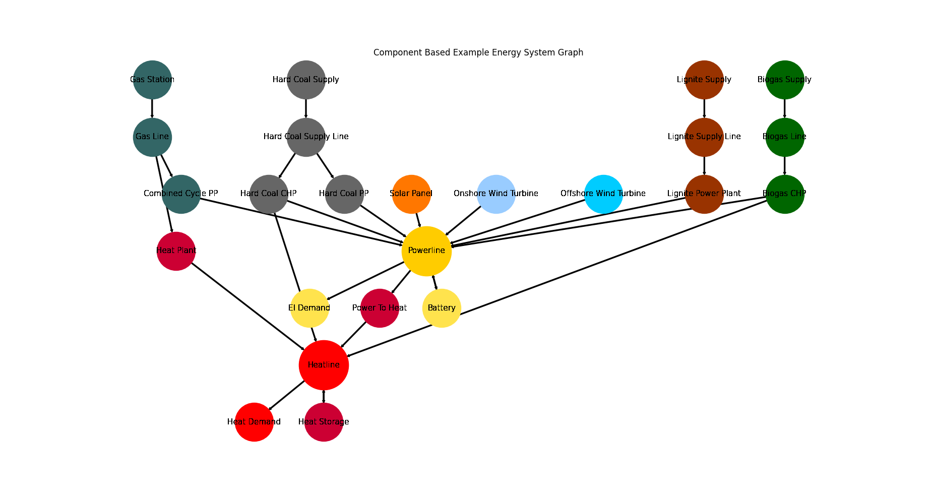
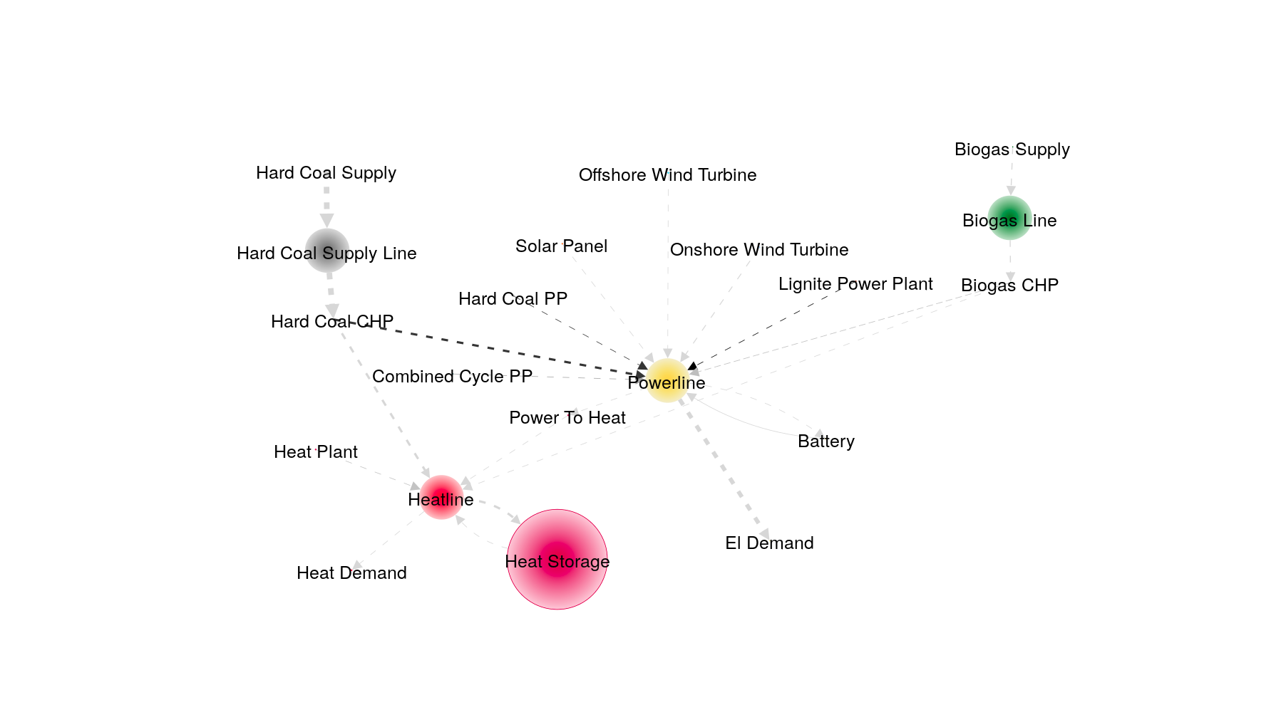
Generic Graph
The system model used for the TransC/E Combinatinos can be seen below:
Optimization Results
The most relevant CompCnE results are listed below. By convention, tessif uses
dynamic dimensioning to allow for different scales of amount of energy
transferred. The current conventions can be seen/adjusted via
tessif.frused.configurations and are as follows for the results below:
MW– for energy flows and installed power capacities
MWh– for amounts of energy and installed storage capacities
EUR– for costs
t_CO2– for emissions (tonns CO2 equivalent)
Commitment
The CompC results generated using the using the respective script, are as follows:
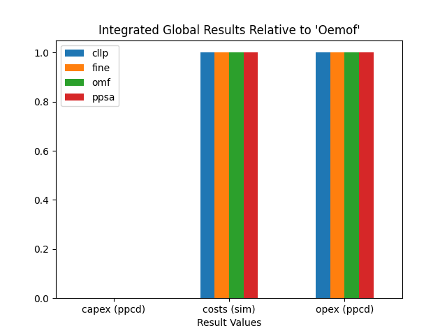
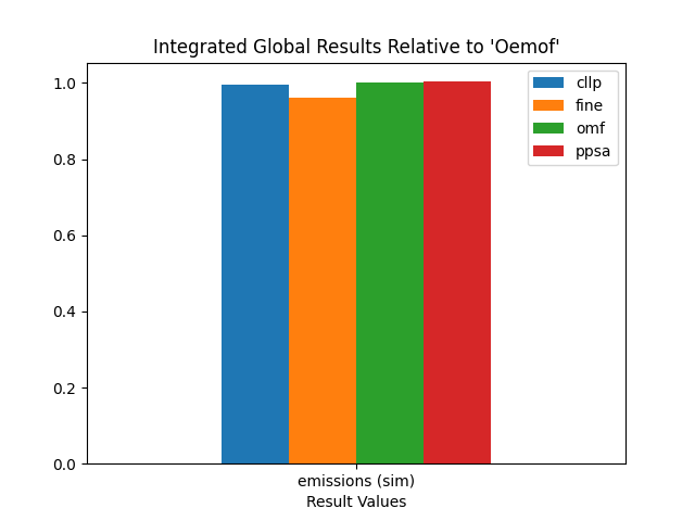
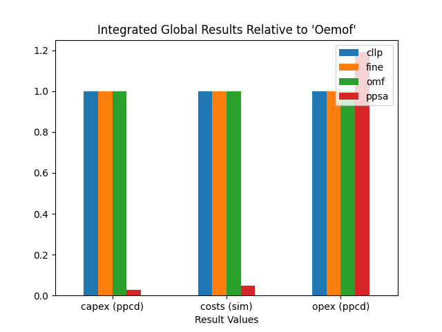
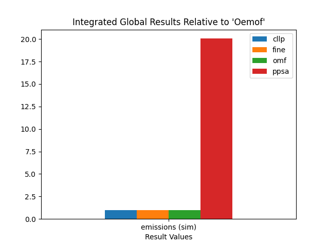
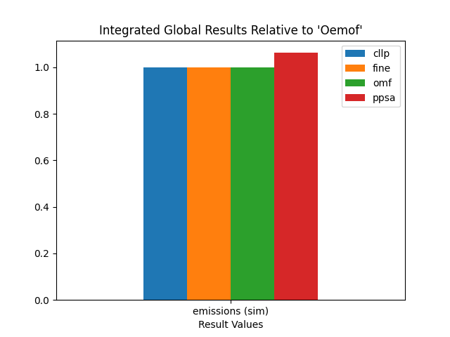
Integrated Global Results
IGR [€ or t_CO2] |
cllp |
fine |
omf |
ppsa |
capex (ppcd) |
0 |
0 |
0 |
0 |
costs (sim) |
688509346 |
688283345 |
688509325 |
688509325 |
emissions (sim) |
6778376 |
6542108 |
6815007 |
6838219 |
opex (ppcd) |
688509352 |
688283344 |
688509325 |
688509325 |
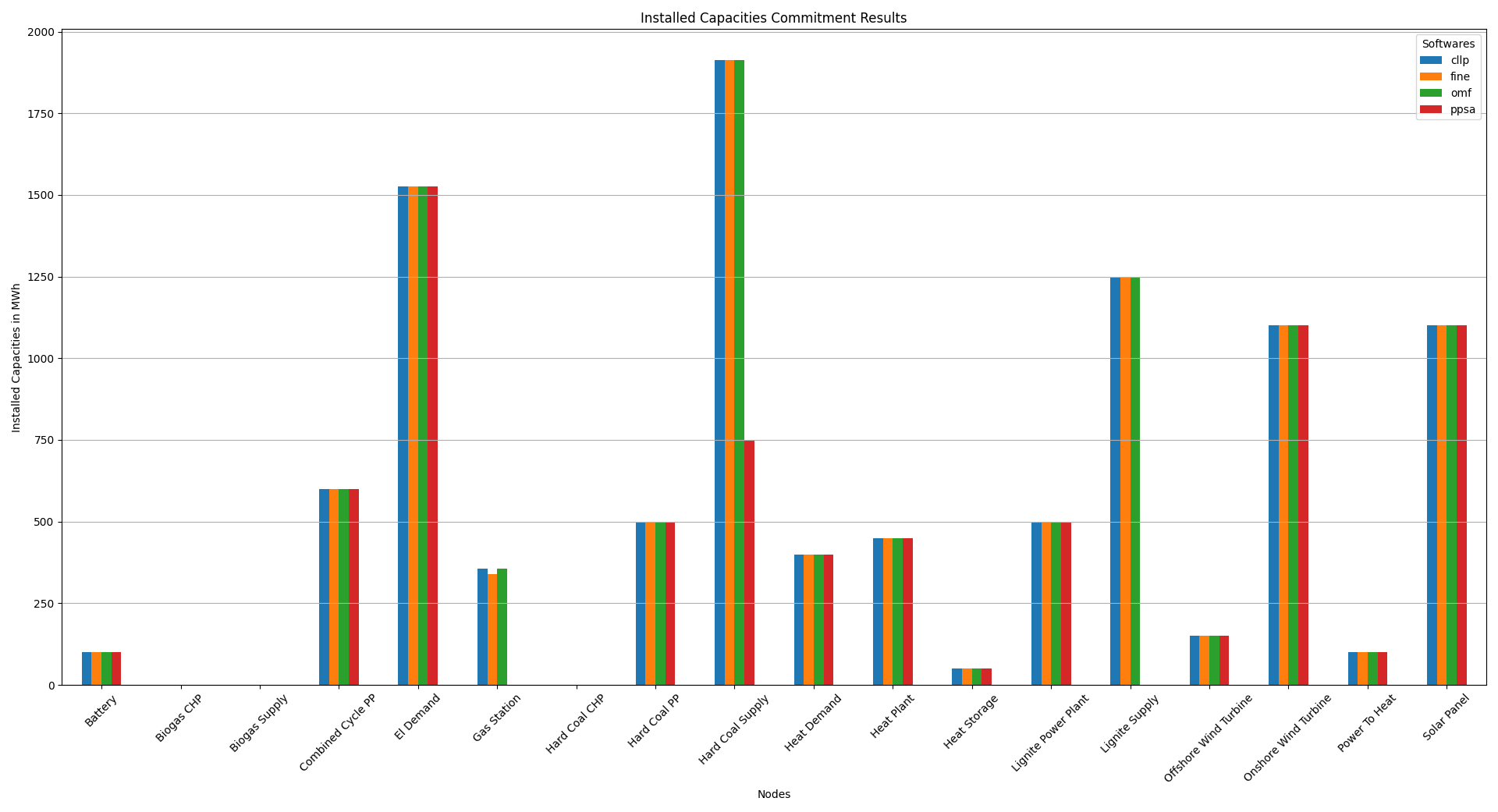
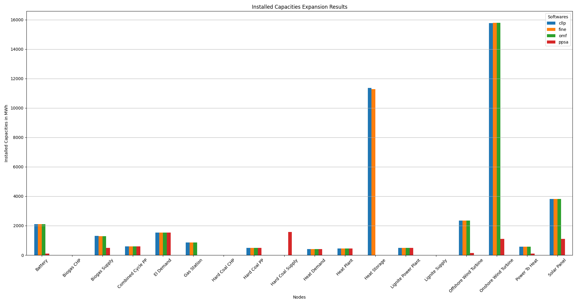
Installed Capacities
Capacity [MW or MWh] |
cllp |
fine |
omf |
ppsa |
Battery |
100 |
100 |
100 |
100 |
Biogas CHP |
[250.0, 200.0] |
[200.0, 250.0] |
[200, 250] |
[250.0, 200.0] |
Biogas Line |
variable |
variable |
variable |
variable |
Biogas Supply |
0 |
0 |
0 |
0 |
Combined Cycle PP |
600 |
600 |
600 |
600 |
El Demand |
1526 |
1526 |
1526 |
1526 |
Gas Line |
variable |
variable |
variable |
variable |
Gas Station |
357 |
340 |
357 |
variable |
Hard Coal CHP |
[300.0, 300.0] |
[300.0, 300.0] |
[300, 300] |
[300.0, 300.0] |
Hard Coal PP |
500 |
500 |
500 |
500 |
Hard Coal Supply |
1912 |
1912 |
1912 |
750 |
Hard Coal Supply Line |
variable |
variable |
variable |
variable |
Heat Demand |
399 |
399 |
399 |
399 |
Heat Plant |
450 |
450 |
450 |
450 |
Heat Storage |
50 |
50 |
50 |
50 |
Heatline |
variable |
variable |
variable |
variable |
Lignite Power Plant |
500 |
500 |
500 |
500 |
Lignite Supply |
1250 |
1250 |
1250 |
variable |
Lignite Supply Line |
variable |
variable |
variable |
variable |
Offshore Wind Turbine |
150 |
150 |
150 |
150 |
Onshore Wind Turbine |
1100 |
1100 |
1100 |
1100 |
Power To Heat |
100 |
100 |
100 |
100 |
Powerline |
variable |
variable |
variable |
variable |
Solar Panel |
1100 |
1100 |
1100 |
1100 |
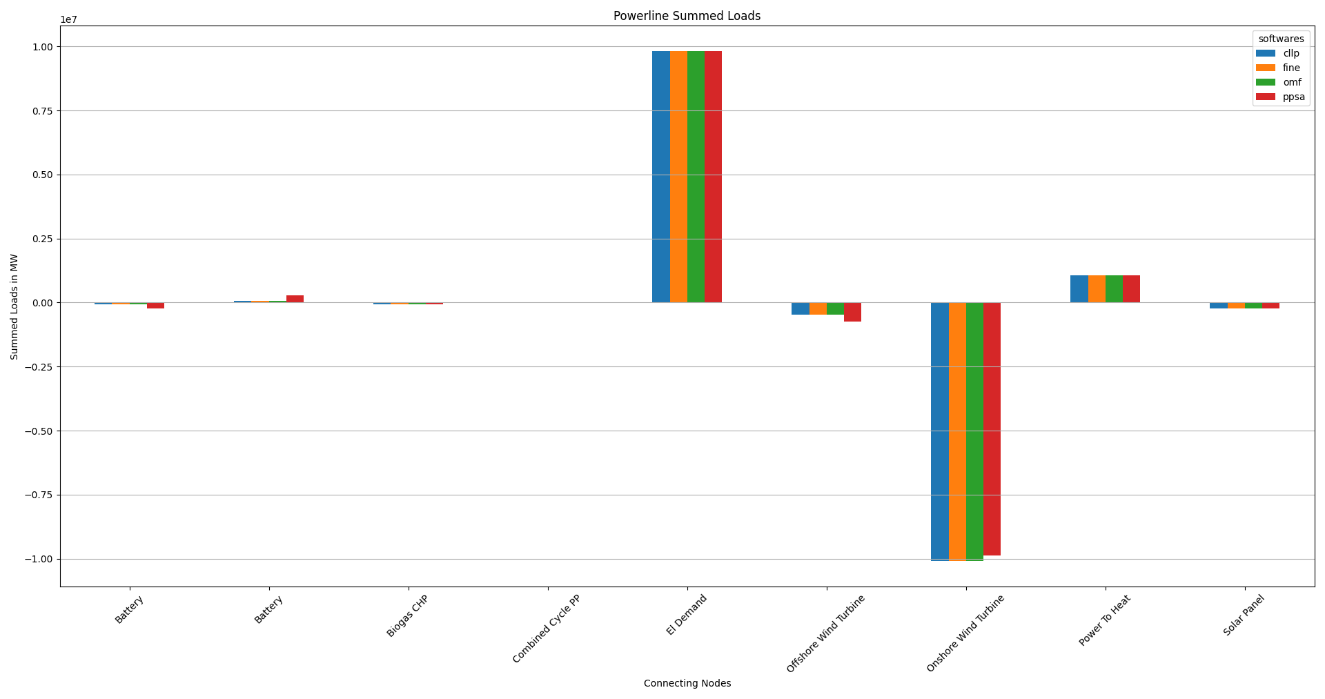
Powerline Results
TODO intro text here
Summed Loads
Load-Powerline [MW] |
cllp |
fine |
omf |
ppsa |
Battery |
-59184 |
-59142 |
-59142 |
-242275 |
Battery |
69736 |
69681 |
69681 |
290281 |
Biogas CHP |
-66772 |
-66470 |
-66470 |
-73816 |
Combined Cycle PP |
-11270 |
-11512 |
-11512 |
-18191 |
El Demand |
9809506 |
9809506 |
9809506 |
9809506 |
Hard Coal CHP |
0 |
0 |
0 |
0 |
Hard Coal PP |
0 |
0 |
0 |
0 |
Lignite Power Plant |
0 |
0 |
0 |
0 |
Offshore Wind Turbine |
-480373 |
-479668 |
-479668 |
-733059 |
Onshore Wind Turbine |
-10089236 |
-10090424 |
-10090424 |
-9880008 |
Power To Heat |
1069849 |
1070091 |
1070091 |
1075836 |
Solar Panel |
-242253 |
-242060 |
-242060 |
-228272 |
Inflows are negative, outflows positive. Connected zero-flow nodes are not shown:
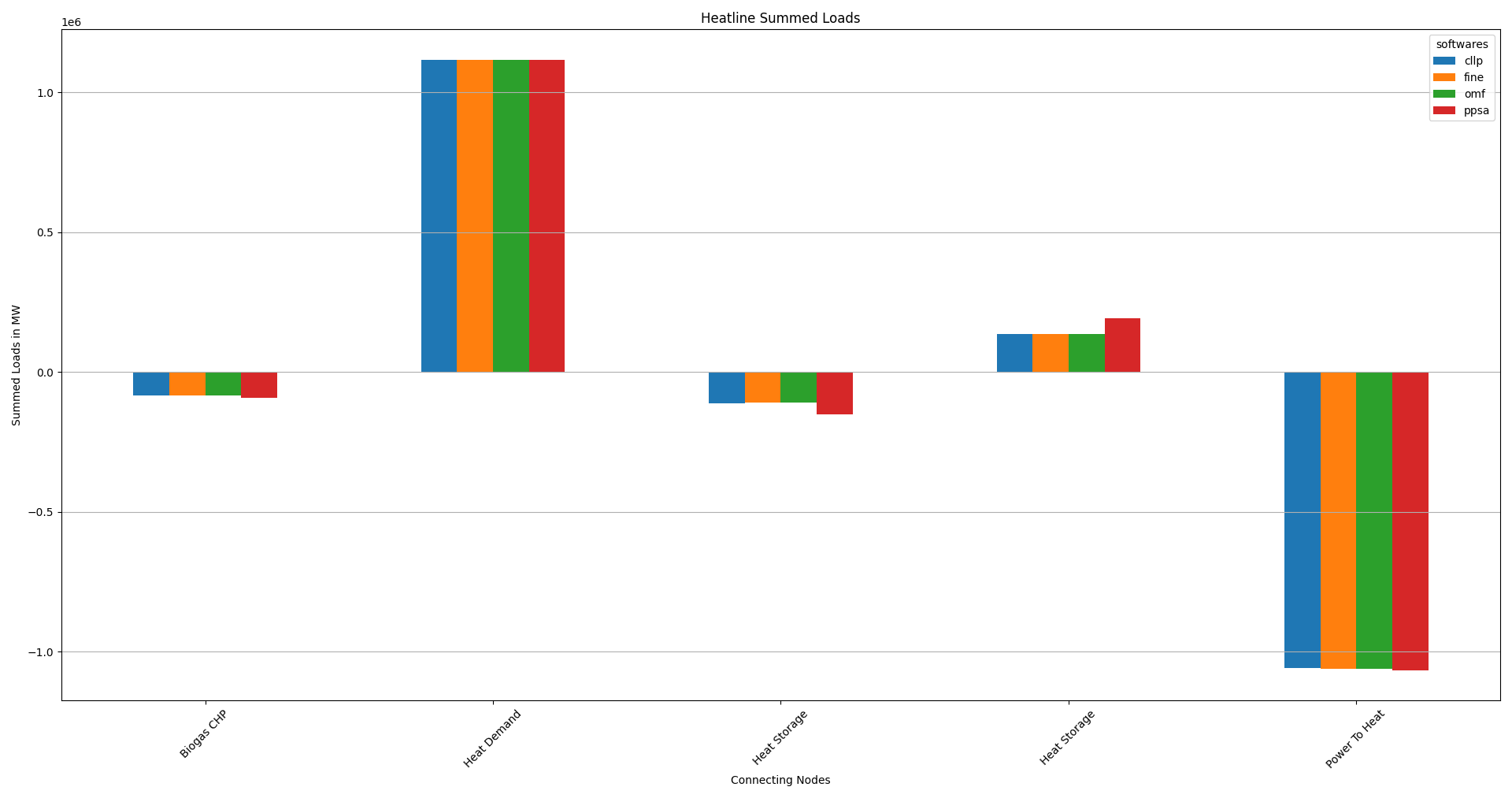
Heatline Results
TODO intro text here
Summed Heat Loads
Load-Heatline [MW] |
cllp |
fine |
omf |
ppsa |
Biogas CHP |
-83465 |
-83088 |
-83088 |
-92271 |
Hard Coal CHP |
0 |
0 |
0 |
0 |
Heat Demand |
1116162 |
1116162 |
1116162 |
1116162 |
Heat Plant |
0 |
0 |
0 |
0 |
Heat Storage |
-110220 |
-109928 |
-109928 |
-150745 |
Heat Storage |
136673 |
136245 |
136245 |
191931 |
Power To Heat |
-1059150 |
-1059390 |
-1059390 |
-1065077 |
Inflows are negative, outflows positive. Connected zero-flow nodes are not shown:
Expansion
The CompC.congestions results generated using the using the respective script, are as follows:
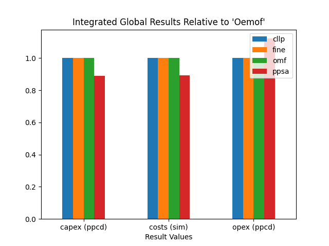
Integrated Global Results
IGR [€ or t_CO2] |
cllp |
fine |
omf |
ppsa |
capex (ppcd) |
41554917514 |
41554976118 |
41554977878 |
1132235997 |
costs (sim) |
42289121225 |
42289118279 |
42289118239 |
2062636560 |
emissions (sim) |
250000 |
250000 |
250000 |
5014819 |
opex (ppcd) |
734204228 |
734140364 |
734140364 |
874603138 |
Installed Capacities
Capacity [MW or MWh] |
cllp |
fine |
omf |
ppsa |
Battery |
2104 |
2104 |
2104 |
100 |
Biogas CHP,”[649.6665625, 519.73325]”,”[516.213, 645.266]”,”[516.21323, 645.26654]”,”[250.0, 200.0]” |
||||
Biogas Line |
variable |
variable |
variable |
variable |
Biogas Supply |
1299 |
1290 |
1290 |
500 |
Combined Cycle PP |
600 |
600 |
600 |
600 |
El Demand |
1526 |
1526 |
1526 |
1526 |
Gas Line |
variable |
variable |
variable |
variable |
Gas Station |
847 |
852 |
852 |
variable |
Hard Coal CHP,”[300.0, 300.0]”,”[300.0, 300.0]”,”[300.0, 300.0]”,”[630.73628, 630.73628]” |
||||
Hard Coal PP |
500 |
500 |
500 |
500 |
Hard Coal Supply |
0 |
0 |
0 |
1576 |
Hard Coal Supply Line |
variable |
variable |
variable |
variable |
Heat Demand |
399 |
399 |
399 |
399 |
Heat Plant |
450 |
450 |
450 |
450 |
Heat Storage |
11357 |
11272 |
11272.2.3391 |
113391.86 |
Heatline |
variable |
variable |
variable |
variable |
Lignite Power Plant |
500 |
500 |
500 |
500 |
Lignite Supply |
0 |
0 |
0 |
variable |
Lignite Supply Line |
variable |
variable |
variable |
variable |
Offshore Wind Turbine |
2347 |
2346 |
2346 |
150 |
Onshore Wind Turbine |
15776 |
15787 |
15787 |
1100 |
Power To Heat |
576 |
576 |
576 |
99 |
Powerline |
variable |
variable |
variable |
variable |
Solar Panel |
3811 |
3809 |
3809 |
1100 |
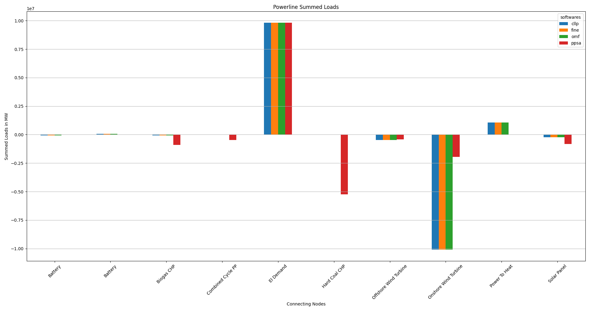
Powerline Results
TODO intro text here
Summed Loads
Load-Powerline [MW] |
cllp |
fine |
omf |
ppsa |
Battery |
-59184 |
-59142 |
-59142 |
-16594 |
Battery |
69736 |
69681 |
69681 |
19032 |
Biogas CHP |
-66772 |
-66470 |
-66470 |
-901176 |
Combined Cycle PP |
-11270 |
-11512 |
-11512 |
-460928 |
El Demand |
9809506 |
9809506 |
9809506 |
9809506 |
Hard Coal CHP |
0 |
0 |
0 |
-5252800 |
Hard Coal PP |
0 |
0 |
0 |
0 |
Lignite Power Plant |
0 |
0 |
0 |
0 |
Offshore Wind Turbine |
-480373 |
-479668 |
-479668 |
-412888 |
Onshore Wind Turbine |
-10089236 |
-10090424 |
-10090424 |
-1959677 |
Power To Heat |
1069849 |
1070091 |
1070091 |
0 |
Solar Panel |
-242253 |
-242060 |
-242060 |
-824472 |
Inflows are negative, outflows positive. Connected zero-flow nodes are not shown:
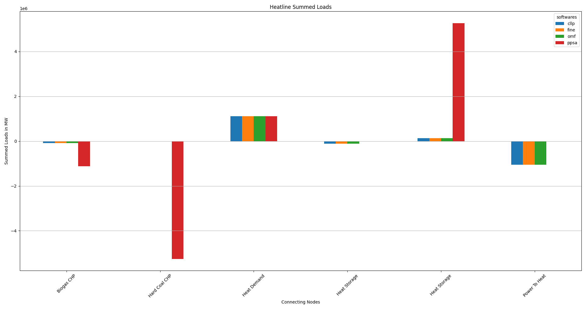
Heatline Results
TODO intro text here
Summed Heat Loads
Load-Heatline [MW] |
cllp |
fine |
omf |
ppsa |
Biogas CHP |
-83465 |
-83088 |
-83088 |
-1126470 |
Hard Coal CHP |
0 |
0 |
0 |
-5252800 |
Heat Demand |
1116162 |
1116162 |
1116162 |
1116162 |
Heat Plant |
0 |
0 |
0 |
0 |
Heat Storage |
-110220 |
-109928 |
-109928 |
0 |
Heat Storage |
136673 |
136245 |
136245 |
5263108 |
Power To Heat |
-1059150 |
-1059390 |
-1059390 |
0 |
Inflows are negative, outflows positive. Connected zero-flow nodes are not shown:
Modified_Expansion
The CompE results generated using the using the respective script, are as follows:
Integrated Global Results
IGR [€ or t_CO2] |
cllp |
fine |
omf |
ppsa |
capex (ppcd) |
41554917514 |
41554976118 |
41554977878 |
36904768288 |
costs (sim) |
42289121225 |
42289118279 |
42289118239 |
37727776780 |
emissions (sim) |
250000 |
250000 |
250000 |
265508 |
opex (ppcd) |
734204228 |
734140364 |
734140364 |
823007841 |
Installed Capacities
Capacity [MW or MWh] |
cllp |
fine |
omf |
ppsa |
Battery |
2104 |
2104 |
2104 |
100 |
Biogas CHP,”[649.6665625, 519.73325]”,”[516.213, 645.266]”,”[516.21323, 645.26654]”,”[250.0, 200.0]” |
||||
Biogas Line |
variable |
variable |
variable |
variable |
Biogas Supply |
1299 |
1290 |
1290 |
500 |
Combined Cycle PP |
600 |
600 |
600 |
600 |
El Demand |
1526 |
1526 |
1526 |
1526 |
Gas Line |
variable |
variable |
variable |
variable |
Gas Station |
847 |
852 |
852 |
variable |
Hard Coal CHP,”[300.0, 300.0]”,”[300.0, 300.0]”,”[300.0, 300.0]”,”[630.73628, 630.73628]” |
||||
Hard Coal PP |
500 |
500 |
500 |
500 |
Hard Coal Supply |
0 |
0 |
0 |
1576 |
Hard Coal Supply Line |
variable |
variable |
variable |
variable |
Heat Demand |
399 |
399 |
399 |
399 |
Heat Plant |
450 |
450 |
450 |
450 |
Heat Storage |
11357 |
11272 |
11272.2.3391 |
113391.86 |
Heatline |
variable |
variable |
variable |
variable |
Lignite Power Plant |
500 |
500 |
500 |
500 |
Lignite Supply |
0 |
0 |
0 |
variable |
Lignite Supply Line |
variable |
variable |
variable |
variable |
Offshore Wind Turbine |
2347 |
2346 |
2346 |
150 |
Onshore Wind Turbine |
15776 |
15787 |
15787 |
1100 |
Power To Heat |
576 |
576 |
576 |
99 |
Powerline |
variable |
variable |
variable |
variable |
Solar Panel |
3811 |
3809 |
3809 |
1100 |
Powerline Results
TODO intro text here
Summed Loads
Load-Powerline [MW] |
cllp |
fine |
omf |
ppsa |
Battery |
-59184 |
-59142 |
-59142 |
-242275 |
Battery |
69736 |
69681 |
69681 |
290281 |
Biogas CHP |
-66772 |
-66470 |
-66470 |
-73816 |
Combined Cycle PP |
-11270 |
-11512 |
-11512 |
-18191 |
El Demand |
9809506 |
9809506 |
9809506 |
9809506 |
Hard Coal CHP |
0 |
0 |
0 |
0 |
Hard Coal PP |
0 |
0 |
0 |
0 |
Lignite Power Plant |
0 |
0 |
0 |
0 |
Offshore Wind Turbine |
-480373 |
-479668 |
-479668 |
-733059 |
Onshore Wind Turbine |
-10089236 |
-10090424 |
-10090424 |
-9880008 |
Power To Heat |
1069849 |
1070091 |
1070091 |
1075836 |
Solar Panel |
-242253 |
-242060 |
-242060 |
-228272 |
Inflows are negative, outflows positive. Connected zero-flow nodes are not shown:
Heatline Results
TODO intro text here
Summed Heat Loads
Load-Heatline [MW] |
cllp |
fine |
omf |
ppsa |
Biogas CHP |
-83465 |
-83088 |
-83088 |
-92271 |
Hard Coal CHP |
0 |
0 |
0 |
0 |
Heat Demand |
1116162 |
1116162 |
1116162 |
1116162 |
Heat Plant |
0 |
0 |
0 |
0 |
Heat Storage |
-110220 |
-109928 |
-109928 |
-150745 |
Heat Storage |
136673 |
136245 |
136245 |
191931 |
Power To Heat |
-1059150 |
-1059390 |
-1059390 |
-1065077 |
Inflows are negative, outflows positive. Connected zero-flow nodes are not shown:
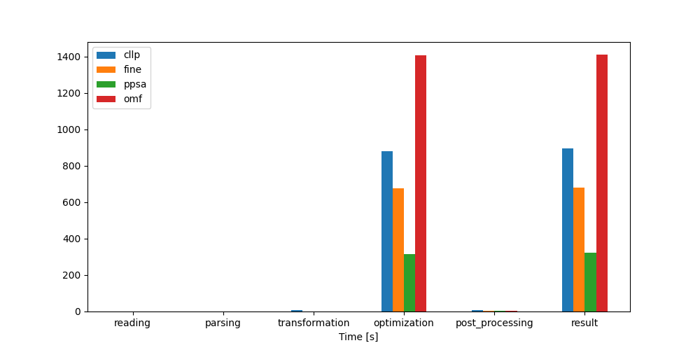
Computationel Ressources Used
Among the Comp combinations the CompE scenario is the most time
consuming. Due to the relatively long timeframe optimized,
Tessif added ressource consumption is negligable:
Timing Results
Time [s] |
cllp |
fine |
ppsa |
omf |
reading |
0.2 |
0.2 |
0.2 |
0.2 |
parsing |
0.3 |
0.2 |
0.2 |
0.2 |
transformation |
6.7 |
0.1 |
1.9 |
0.0 |
optimization |
880.7 |
676.4 |
316.1 |
1405.8 |
post_processing |
6.1 |
3.5 |
2.5 |
3.1 |
result |
894.0 |
680.5 |
321.0 |
1409.4 |
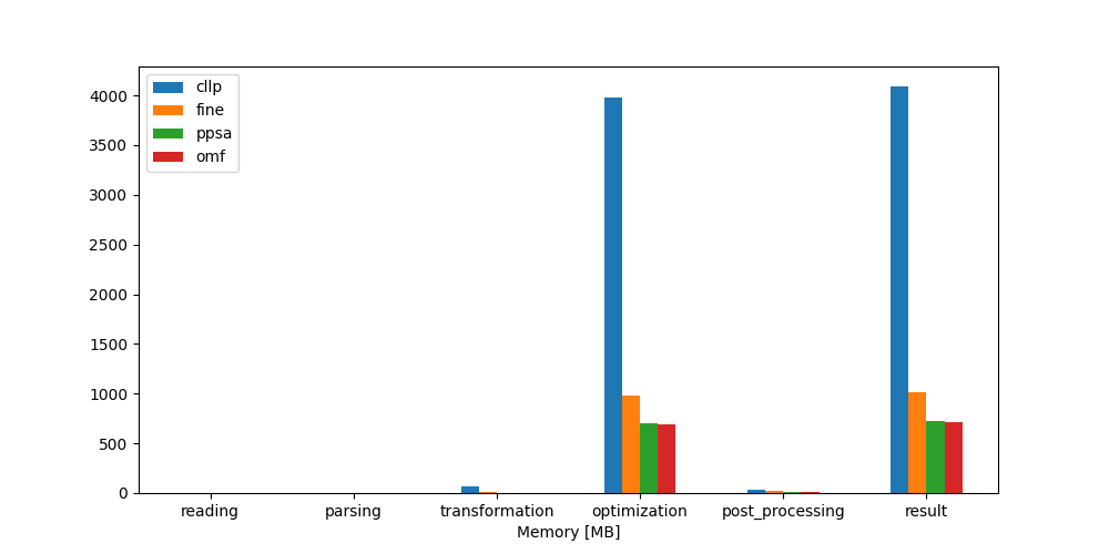
Memory Results
Memory [MB] |
cllp |
fine |
ppsa |
omf |
reading |
3.0 |
3.0 |
3.0 |
3.0 |
parsing |
1.0 |
1.0 |
1.0 |
1.0 |
transformation |
62.0 |
16.0 |
3.0 |
1.0 |
optimization |
3984.0 |
979.0 |
707.0 |
690.0 |
post_processing |
36.0 |
18.0 |
13.0 |
15.0 |
result |
4087.0 |
1017.0 |
727.0 |
710.0 |
Advanced Graphs
Following sections show the advanced graph representations of the three
model-scenario-combinations showing the greatest differences, i.e
the Expansion and the Modified-Expansion combinations. Since result
variation in between softwares others then Pypsa is low, only the
Oemof graph is shown for the Expansion combinations.
To facilitate inter software comparison, the advanced graphs below, are drawn
relative to the installed capacity and net energy flow of the demand component
"El Demand".
Expansion
Oemof

PyPSA
The Integrated Global Results
indicate, that the PyPSA results differ significantly. An initial attempt
to relate node size to the installed capacity and net energy flow of the demand
component "El Demand" fails, since the resulting size of the
Heat Storage component is too large. Thus the advanced system
visualization below is plotted relating node size to the installed capacity of
the Heat Storage component.
Modified_Expansion
Modifying the PyPSA system model scenario combination, leads to
optimization results closer to that of the other softwares. The advanced
graph below is therfor again drawn relative to the installed capacity and net
energy flow of the demand component "El Demand".
PyPSA

Key Observations
Comparing the above advanced graph visulaizations, three main differences are easily observed between the three scenarios:
The non-modified expansion combination of
PyPSAdiffers largely. The"Heat Storage"component is used extensively indicating that the"Hard Coal CHP"component is used to provide power and electricity, while the component is used to store uneeded heat.The advanced graph visualization of the modified
PyPSAexpansion combination resembles that ofOemofmuch closer in comparison to the non-modified variation.For the optimal solution Onshore, Solar, Offshore and Heat Storage are used the most having relatively large installed capacities compared to the compartively low characteristic value / capacity factor.
Key Conclusions
The Key Goal could be served in the sense of developing a reference supply system model in conjunction with two relevant and contemporary scenario formulations to test out the modelling softwares
Calliope,Fine,OemofandPypsa.All of the 5 aims (Thesis-> Method -> Modelling -> MSC Selection ) formulated, with regards to component focused model behaviour, were successfully addressed:
Integration of volatile renewable energy sources into an existing system:
The components
Solar Panel,Onshore Wind TurbineandOffshore Wiind Turbinerepresent succesfully integrated, volatile renewable energy sources, of which the maximum power produced is constraint via hourly resolved load profiles as discussed in Reimer, Ammon in Subsection - 3.2.4 and Subsection - 3.2.5
Integration of energy storage technologies into an existing system:
The components
BatteryandHeat Storagerepresent successfully integrated electrical and thermal energy storage components respectively. They are parameterized in accordance to contemporary tecnical specifications as discussed in Reimer, Ammon Subsection - 3.2.10
Year-round, hourly-resolved energy demands based on ambient climatic conditions:
The components
El DemandandHeat Demandrepresent succesfully modeled, hourly-resolved energy demands based on real world considerations as laid out in Reimer, Ammon Subsection 3.2.1
Cost optimally dispatching energy sources to meet the system’s demand:
The use case is succesfully modelled via the
CompCcombination of which the generic graph representation can be seen above.The results are evaluated using the codes shown in the respective code section and shown above.
Reaching emission-goals cost optimally on given constraints, potentially expanding or adding certain low-emission components.
The use case is succesfully modelled via the
CompEcombination of which the generic graph representation can be seen above.The results are evaluated using the codes shown in the respective code section and shown above.
In addition to that following insights were gained with regards to the softwares used:
Given the same input it is possible, but not necessarily directly implied, to produce the exact same results on relatively large and complex energy supply system models for all softwares investigated.
Emission constraint expansion problems reveal software specific differences more clearly in comparison to pure commitment problems.
Emission allocation differs between softwares. Leading to potentially large differences as demonstrated by the unmodified expansion results.
The possibility to assign emissions to storage and sector coupling components, in particular, varies significantly between softwares.
See also Reimer, Ammon - Subsections 4.3.2 and 4.3.3 for an in detail discussed comparison between
oemofandPyPsain this regard.Storage parameterization varies significantly between softwares. These constitute mainly of:
Initial State of Charge
Emission allocation – Differences beeing in both, the possibility to allocate emissions in the first place, and the option to which energy flow allocation is possible (inflow, outflow or both).
Cost allocation – Difference beeing wheter the costs are allocatable energy flow specific (inflow, outflow or both)l or only to State of Charge differences between first and final time step.
Internal represtation differences in cost and emission allocation can be compnensated without actually altering the defacto interpreation of the input, if so desired. Further more this alteration is done relatively simple using tessif, as is demonstrated in the respective code snippet below.
Tessif facilitates comparison, by allowing straight forward energy supply sytem model creation, transformation, optimization, post-processing, result comparison and visualization as demonstrated by the code with which the abov results were generated.
On comparitevly medium to large timeframes, like the above 8760 hourly steps, Tessif introduced need of computational ressources is negligable (see figures in section Computationel Ressources Used).
Comparing the computational ressourcess needed between softwares on the above model-scenario-combinations, it seems as though tessif-pypsa is generally more efficient than tessif-fine, which is more efficient than tessif-calliope, which in turn is more efficient than tessif-oemof.