Discussion/Overview
Generic Graph
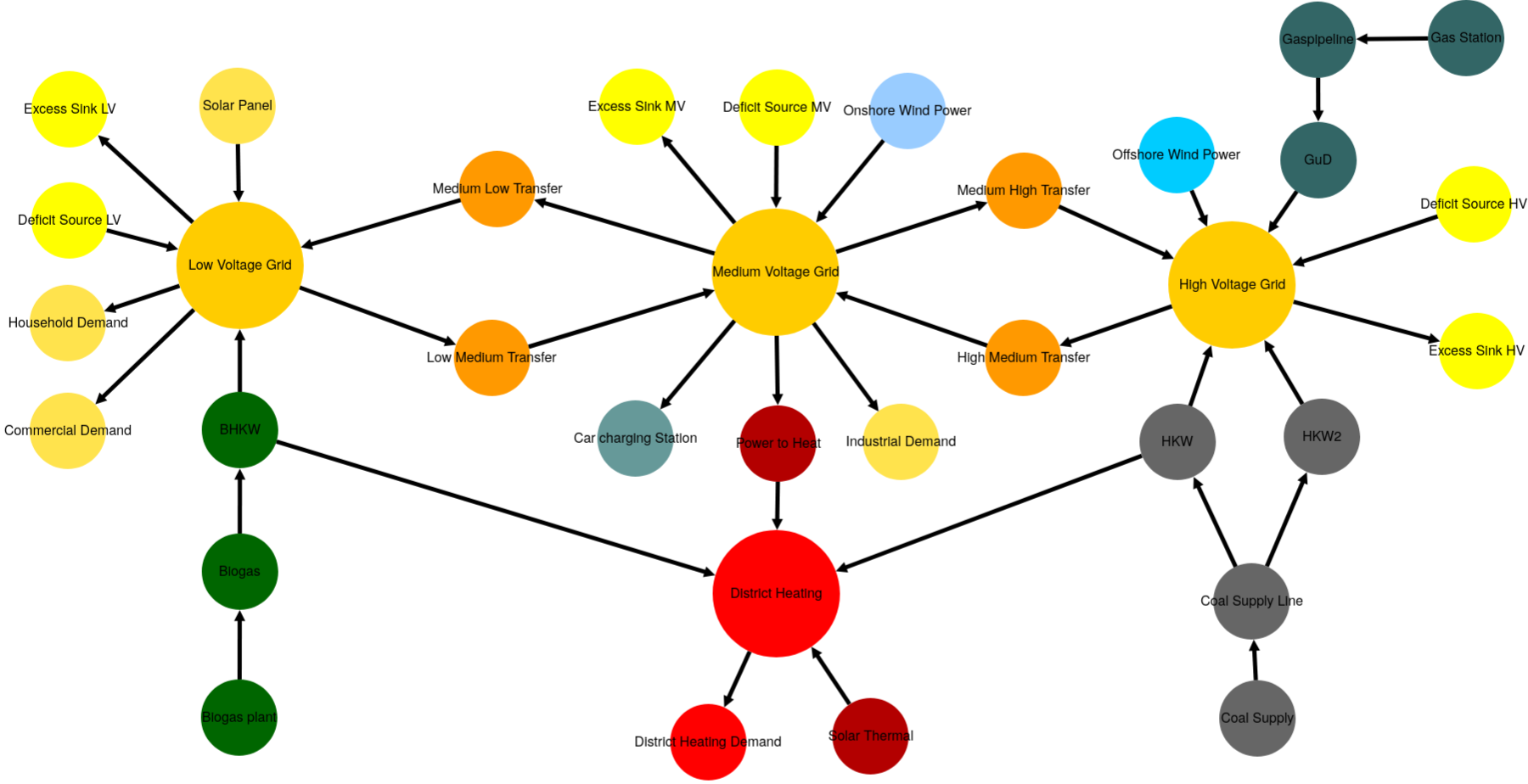
The system model used for the TransC/E Combinatinos can be seen below:
Optimization Results
The most relevant TransCnE results are listed below. By convention, tessif uses
dynamic dimensioning to allow for different scales of amount of energy
transferred. The current conventions can be seen/adjusted via
tessif.frused.configurations and are as follows for the results below:
MW– for energy flows and installed power capacities
MWh– for amounts of energy and installed storage capacities
EUR– for costs
t_CO2– for emissions (tonns CO2 equivalent)
No Congestion Commitment
The CompC-no-congestions results generated using the using the respective script, are as follows:
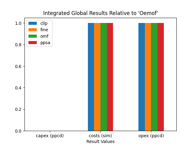
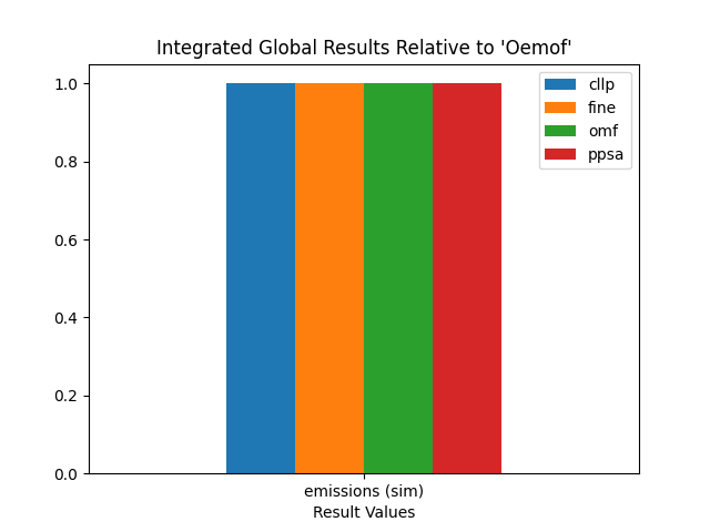
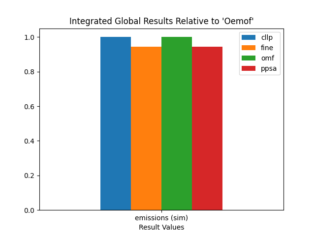
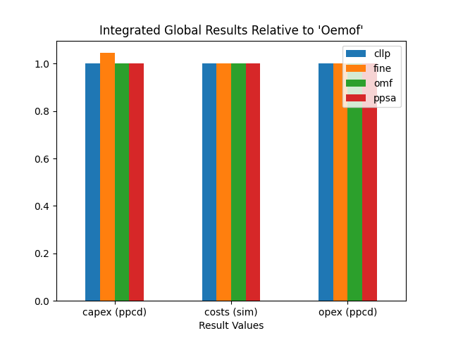
Integrated Global Results
IGR [€ or t_CO2] |
cllp |
fine |
omf |
ppsa |
capex (ppcd) |
0 |
0 |
0 |
0 |
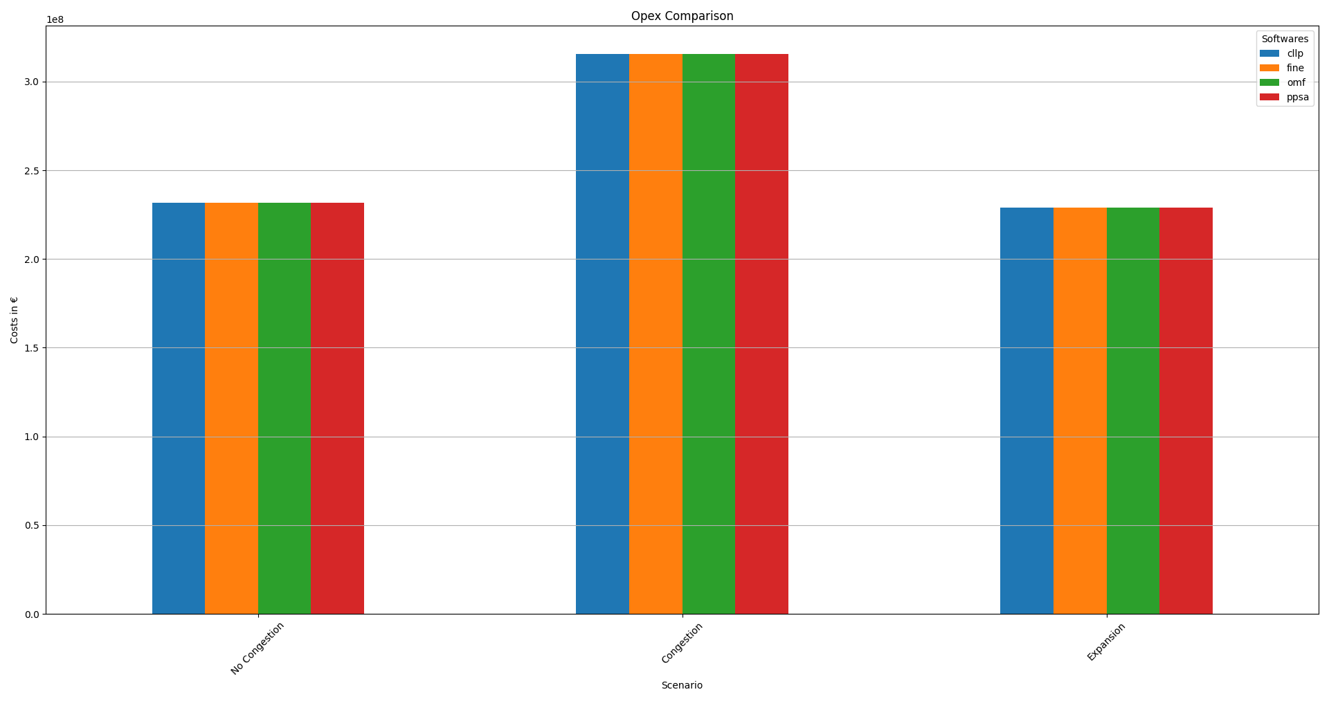
costs (sim) |
231793808 |
231793807 |
231793807 |
231793807 |
emissions (sim) |
482759 |
482759 |
482759 |
482759 |
opex (ppcd) |
231793807 |
231793807 |
231793806 |
231793807 |
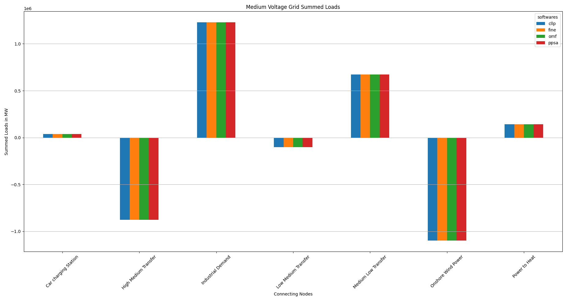
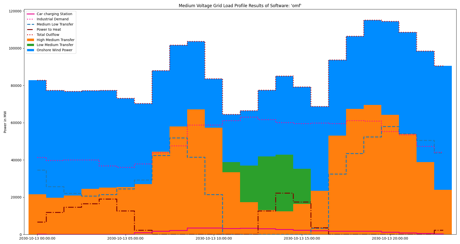
Medium Voltage Grid Loads Results
Comparing the integrated global results from above as well as the detailed numerical load results of the high, medium and low voltage grid busses, shows, that the different softwares all solve the TransC model-scenario-combination quite similarly.
The representative summed loads bar plot as well as the load profile plot for software “oemof” are shown below.
Summed Loads
Load-Medium Voltage Grid [MW] |
cllp |
fine |
omf |
ppsa |
Car charging Station |
37026 |
37026 |
37026 |
37026 |
Deficit Source MV |
0 |
0 |
0 |
0 |
Excess Sink MV |
0 |
0 |
0 |
0 |
High Medium Transfer |
-849604 |
-849604 |
-849604 |
-849604 |
Industrial Demand |
1229008 |
1229008 |
1229008 |
1229008 |
Low Medium Transfer |
-103346 |
-103346 |
-103346 |
-103346 |
Medium High Transfer |
0 |
0 |
0 |
0 |
Medium Low Transfer |
645101 |
645101 |
645101 |
645101 |
Onshore Wind Power |
-1099866 |
-1099866 |
-1099866 |
-1099866 |
Power to Heat |
141680 |
141680 |
141680 |
141680 |
Inflows are negative, outflows positive. Connected zero-flow nodes are not shown:
Load Profile Plot “Oemof”
Deficit Source MV |
High Medium Transfer |
Low Medium Transfer |
Onshore Wind Power |
Car charging Station |
Excess Sink MV |
Industrial Demand |
Medium High Transfer |
Medium Low Transfer |
Power to Heat |
|
2030-10-13 00:00:00 |
0 |
-21530.999 |
0.0 |
-61321.041 |
199.55034 |
0 |
41420.707 |
0 |
34579.956 |
6651.8273 |
2030-10-13 01:00:00 |
0 |
-19679.209 |
0.0 |
-57645.374 |
33.761407 |
0 |
39808.658 |
0 |
25675.673 |
11806.491 |
2030-10-13 02:00:00 |
0 |
-20854.971 |
0.0 |
-55988.777 |
23.179135 |
0 |
40077.333 |
0 |
22120.867 |
14622.369 |
2030-10-13 03:00:00 |
0 |
-24432.298 |
0.0 |
-52771.444 |
23.179135 |
0 |
40077.333 |
0 |
20636.279 |
16466.952 |
2030-10-13 04:00:00 |
0 |
-25190.678 |
0.0 |
-52130.374 |
79.617922 |
0 |
36853.235 |
0 |
21393.545 |
18994.654 |
2030-10-13 05:00:00 |
0 |
-25431.492 |
0.0 |
-47729.758 |
93.727619 |
0 |
36002.431 |
0 |
24427.32 |
12637.772 |
2030-10-13 06:00:00 |
0 |
-26990.02 |
0.0 |
-43383.064 |
912.09003 |
0 |
37927.934 |
0 |
29254.143 |
2278.9176 |
2030-10-13 07:00:00 |
0 |
-44435.758 |
0.0 |
-43520.864 |
1698.7056 |
0 |
43883.56 |
0 |
42374.356 |
0.0 |
2030-10-13 08:00:00 |
0 |
-58020.43 |
0.0 |
-43664.656 |
2192.545 |
0 |
47645.008 |
0 |
51847.533 |
0.0 |
2030-10-13 09:00:00 |
0 |
-60000.0 |
0.0 |
-36630.859 |
3473.0 |
0 |
58750.236 |
0 |
34407.624 |
0.0 |
2030-10-13 10:00:00 |
0 |
-57285.428 |
0.0 |
-26343.783 |
3444.7806 |
0 |
58750.236 |
0 |
21434.195 |
0.0 |
2030-10-13 11:00:00 |
0 |
-33327.749 |
-5472.3418 |
-25663.769 |
3250.7723 |
0 |
61213.088 |
0 |
0.0 |
0.0 |
2030-10-13 12:00:00 |
0 |
-17294.145 |
-19706.517 |
-29453.272 |
3360.1224 |
0 |
63093.812 |
0 |
0.0 |
0.0 |
2030-10-13 13:00:00 |
0 |
-13018.034 |
-28889.815 |
-35624.32 |
3134.3673 |
0 |
61750.438 |
0 |
0.0 |
12647.364 |
2030-10-13 14:00:00 |
0 |
-12406.164 |
-30432.837 |
-42280.663 |
2707.5489 |
0 |
60138.389 |
0 |
0.0 |
22273.726 |
2030-10-13 15:00:00 |
0 |
-16375.402 |
-18844.881 |
-44012.151 |
2234.8741 |
0 |
59601.039 |
0 |
0.0 |
17396.521 |
2030-10-13 16:00:00 |
0 |
-23472.995 |
0.0 |
-45315.261 |
2005.5915 |
0 |
59869.714 |
0 |
3319.4264 |
3593.5244 |
2030-10-13 17:00:00 |
0 |
-53098.587 |
0.0 |
-40621.071 |
1716.3428 |
0 |
59601.039 |
0 |
32402.276 |
0.0 |
2030-10-13 18:00:00 |
0 |
-60000.0 |
0.0 |
-39003.418 |
1758.6718 |
0 |
61213.088 |
0 |
36031.657 |
0.0 |
2030-10-13 19:00:00 |
0 |
-60000.0 |
0.0 |
-45599.848 |
1790.4187 |
0 |
60944.414 |
0 |
42865.016 |
0.0 |
2030-10-13 20:00:00 |
0 |
-60000.0 |
0.0 |
-50297.034 |
1233.0856 |
0 |
55257.462 |
0 |
53806.486 |
0.0 |
2030-10-13 21:00:00 |
0 |
-53983.53 |
0.0 |
-54613.772 |
859.17867 |
0 |
53600.634 |
0 |
54137.489 |
0.0 |
2030-10-13 22:00:00 |
0 |
-38829.106 |
0.0 |
-59652.462 |
509.96367 |
0 |
47376.333 |
0 |
50595.271 |
0.0 |
2030-10-13 23:00:00 |
0 |
-23947.329 |
0.0 |
-66599.384 |
291.26337 |
0 |
44152.235 |
0 |
43792.749 |
2310.4665 |
Inflows are represented as stacked bars, outflows as stacked step plots. Connected zero-flow nodes are not shown:
Redispatch
For the No-Congestion TransC combination no redispatch is needed.
Circulated Energy Transport
For the No-Congestion TransC combination no energy is circulated between
busses to reduce the amount of excess sink fed energy (which is costly).
Congestion Commitment
The CompC.congestions results generated using the using the respective script, are as follows:
Integrated Global Results
IGR [€ or t_CO2] |
cllp |
fine |
omf |
ppsa |
capex (ppcd) |
0 |
0 |
0 |
0 |
costs (sim) |
315601734 |
315601734 |
315601734 |
315601734 |
emissions (sim) |
476089 |
449817 |
476089 |
449817 |
opex (ppcd) |
315601732 |
315601732 |
315601732 |
315601732 |

Medium Voltage Grid Loads Results
Comparing the integrated global results from above as well as the detailed numerical load results of the high, medium and low voltage grid busses, shows, that the different softwares all solve the TransC model-scenario-combination quite similarly.
The representative summed loads bar plot as well as the load profile plot for software “oemof” are shown below.
Summed Loads
Load-Medium Voltage Grid [MW] |
cllp |
fine |
omf |
ppsa |
Car charging Station |
37026 |
37026 |
37026 |
37026 |
Deficit Source MV |
-38460 |
-38460 |
-38460 |
-38460 |
Excess Sink MV |
0 |
0 |
0 |
0 |
High Medium Transfer |
-428888 |
-428888 |
-428888 |
-428888 |
Industrial Demand |
1229008 |
1229008 |
1229008 |
1229008 |
Low Medium Transfer |
-91480 |
-91480 |
-91480 |
-91480 |
Medium High Transfer |
0 |
0 |
0 |
0 |
Medium Low Transfer |
219628 |
219628 |
219628 |
219628 |
Onshore Wind Power |
-1099866 |
-1099866 |
-1099866 |
-1099866 |
Power to Heat |
173033 |
173033 |
173033 |
173033 |
Inflows are negative, outflows positive. Connected zero-flow nodes are not shown:
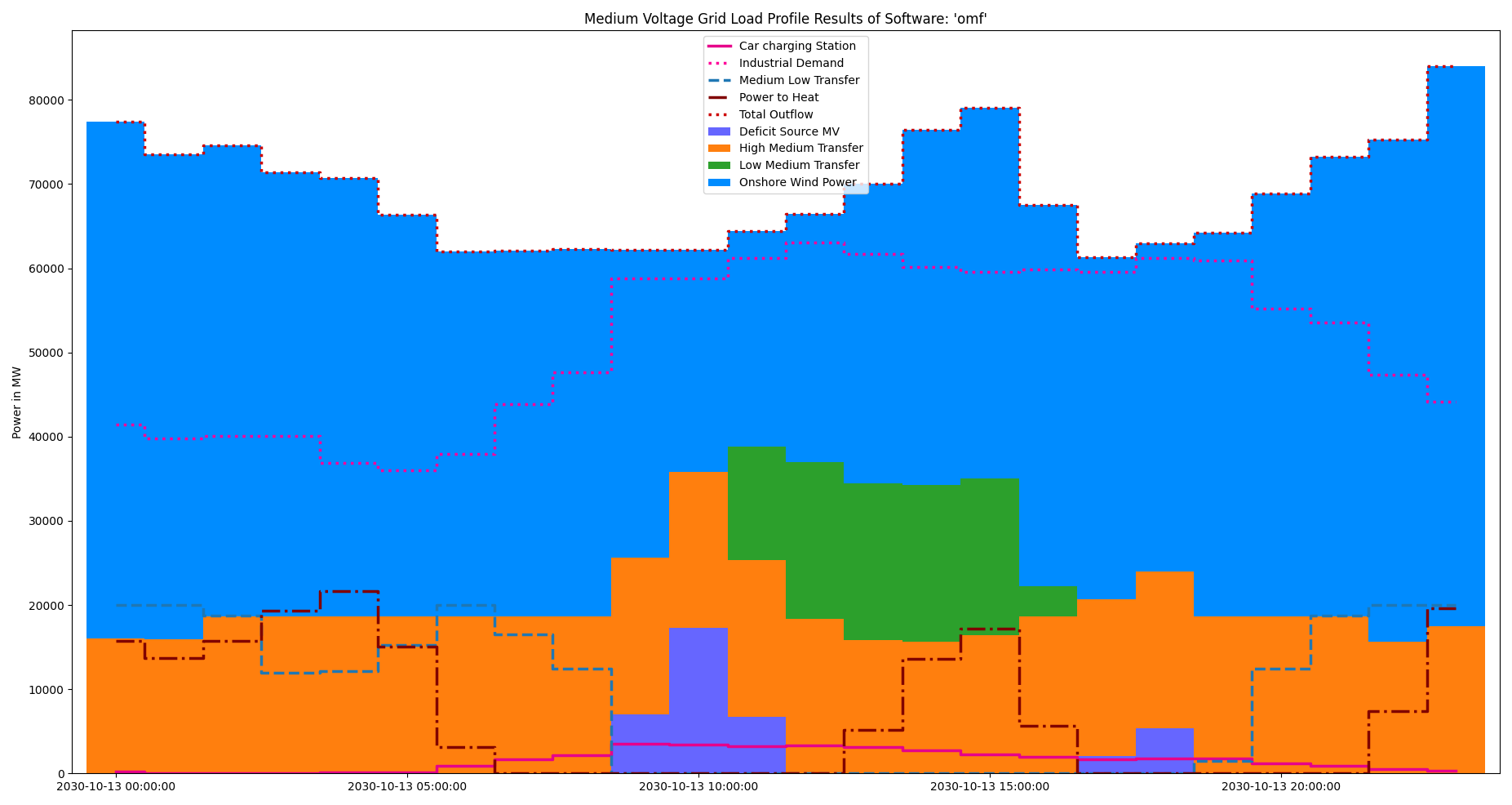
Load Profile Plot “Oemof”
Deficit Source MV |
High Medium Transfer |
Low Medium Transfer |
Onshore Wind Power |
Car charging Station |
Excess Sink MV |
Industrial Demand |
Medium High Transfer |
Medium Low Transfer |
Power to Heat |
|
2030-10-13 00:00:00 |
0.0 |
-16064.385 |
0.0 |
-61321.041 |
199.55034 |
0 |
41420.707 |
0 |
20000.0 |
15765.169 |
2030-10-13 01:00:00 |
0.0 |
-15885.158 |
0.0 |
-57645.374 |
33.761407 |
0 |
39808.658 |
0 |
20000.0 |
13688.112 |
2030-10-13 02:00:00 |
0.0 |
-18600.0 |
0.0 |
-55988.777 |
23.179135 |
0 |
40077.333 |
0 |
18747.566 |
15740.699 |
2030-10-13 03:00:00 |
0.0 |
-18600.0 |
0.0 |
-52771.444 |
23.179135 |
0 |
40077.333 |
0 |
11911.51 |
19359.422 |
2030-10-13 04:00:00 |
0.0 |
-18600.0 |
0.0 |
-52130.374 |
79.617922 |
0 |
36853.235 |
0 |
12172.04 |
21625.482 |
2030-10-13 05:00:00 |
0.0 |
-18600.0 |
0.0 |
-47729.758 |
93.727619 |
0 |
36002.431 |
0 |
15205.815 |
15027.785 |
2030-10-13 06:00:00 |
0.0 |
-18600.0 |
0.0 |
-43383.064 |
912.09003 |
0 |
37927.934 |
0 |
20000.0 |
3143.0399 |
2030-10-13 07:00:00 |
0.0 |
-18600.0 |
0.0 |
-43520.864 |
1698.7056 |
0 |
43883.56 |
0 |
16538.598 |
0.0 |
2030-10-13 08:00:00 |
0.0 |
-18600.0 |
0.0 |
-43664.656 |
2192.545 |
0 |
47645.008 |
0 |
12427.102 |
0.0 |
2030-10-13 09:00:00 |
-6992.3761 |
-18600.0 |
0.0 |
-36630.859 |
3473.0 |
0 |
58750.236 |
0 |
0.0 |
0.0 |
2030-10-13 10:00:00 |
-17251.233 |
-18600.0 |
0.0 |
-26343.783 |
3444.7806 |
0 |
58750.236 |
0 |
0.0 |
0.0 |
2030-10-13 11:00:00 |
-6752.0694 |
-18600.0 |
-13448.022 |
-25663.769 |
3250.7723 |
0 |
61213.088 |
0 |
0.0 |
0.0 |
2030-10-13 12:00:00 |
0.0 |
-18400.663 |
-18600.0 |
-29453.272 |
3360.1224 |
0 |
63093.812 |
0 |
0.0 |
0.0 |
2030-10-13 13:00:00 |
0.0 |
-15807.984 |
-18600.0 |
-35624.32 |
3134.3673 |
0 |
61750.438 |
0 |
0.0 |
5147.4985 |
2030-10-13 14:00:00 |
0.0 |
-15614.484 |
-18600.0 |
-42280.663 |
2707.5489 |
0 |
60138.389 |
0 |
0.0 |
13649.21 |
2030-10-13 15:00:00 |
0.0 |
-16441.798 |
-18600.0 |
-44012.151 |
2234.8741 |
0 |
59601.039 |
0 |
0.0 |
17218.036 |
2030-10-13 16:00:00 |
0.0 |
-18600.0 |
-3632.974 |
-45315.261 |
2005.5915 |
0 |
59869.714 |
0 |
0.0 |
5672.9293 |
2030-10-13 17:00:00 |
-2096.3111 |
-18600.0 |
0.0 |
-40621.071 |
1716.3428 |
0 |
59601.039 |
0 |
0.0 |
0.0 |
2030-10-13 18:00:00 |
-5368.3426 |
-18600.0 |
0.0 |
-39003.418 |
1758.6718 |
0 |
61213.088 |
0 |
0.0 |
0.0 |
2030-10-13 19:00:00 |
0.0 |
-18600.0 |
0.0 |
-45599.848 |
1790.4187 |
0 |
60944.414 |
0 |
1465.0159 |
0.0 |
2030-10-13 20:00:00 |
0.0 |
-18600.0 |
0.0 |
-50297.034 |
1233.0856 |
0 |
55257.462 |
0 |
12406.486 |
0.0 |
2030-10-13 21:00:00 |
0.0 |
-18600.0 |
0.0 |
-54613.772 |
859.17867 |
0 |
53600.634 |
0 |
18753.959 |
0.0 |
2030-10-13 22:00:00 |
0.0 |
-15627.265 |
0.0 |
-59652.462 |
509.96367 |
0 |
47376.333 |
0 |
20000.0 |
7393.4297 |
2030-10-13 23:00:00 |
0.0 |
-17447.163 |
0.0 |
-66599.384 |
291.26337 |
0 |
44152.235 |
0 |
20000.0 |
19603.048 |
Inflows are represented as stacked bars, outflows as stacked step plots. Connected zero-flow nodes are not shown:
Redispatch
For the Congestion TransC combination a small amount of power is
redispatched during 2 of the 24 timesteps as shown below.
Timeseries-High Voltage Grid [MW] |
Redispatch High -> Medium |
2030-10-13 17:00:00 |
2096 |
2030-10-13 18:00:00 |
5368 |
Circulated Energy Transport
For the Congestion TransC combination no energy is circulated between
busses to reduce the amount of excess sink fed energy (which is costly).
Medium and High
Timeseries-Medium Voltage Grid [MW] |
Circulation Medium and High |
Expansion
The TransE results generated using the using the respective script, are as follows:
Integrated Global Results
IGR [€ or t_CO2] |
cllp |
fine |
omf |
ppsa |
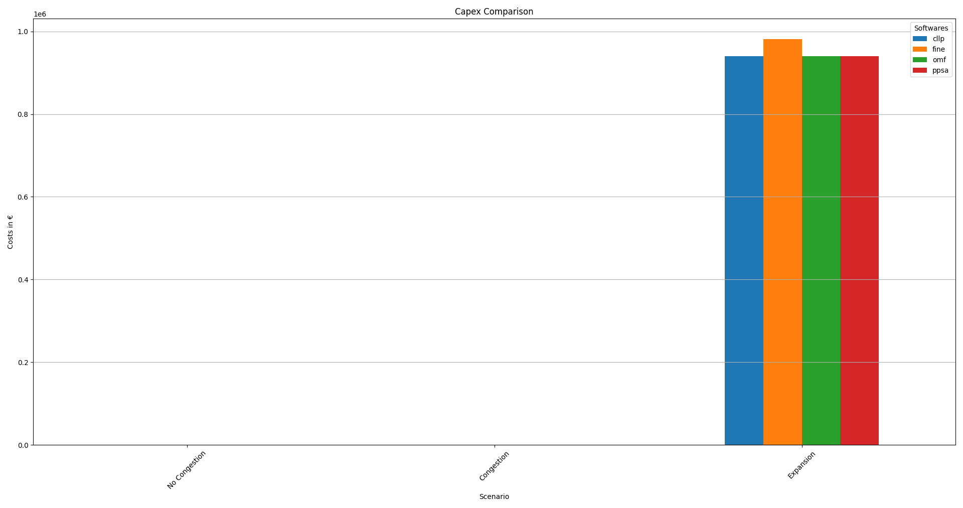
capex (ppcd) |
939554 |
981554 |
939554 |
939554 |
costs (sim) |
229708134 |
229750135 |
229708135 |
229708135 |
emissions (sim) |
484261 |
484261 |
484261 |
484261 |
opex (ppcd) |
228768580 |
228768581 |
228768581 |
228768581 |

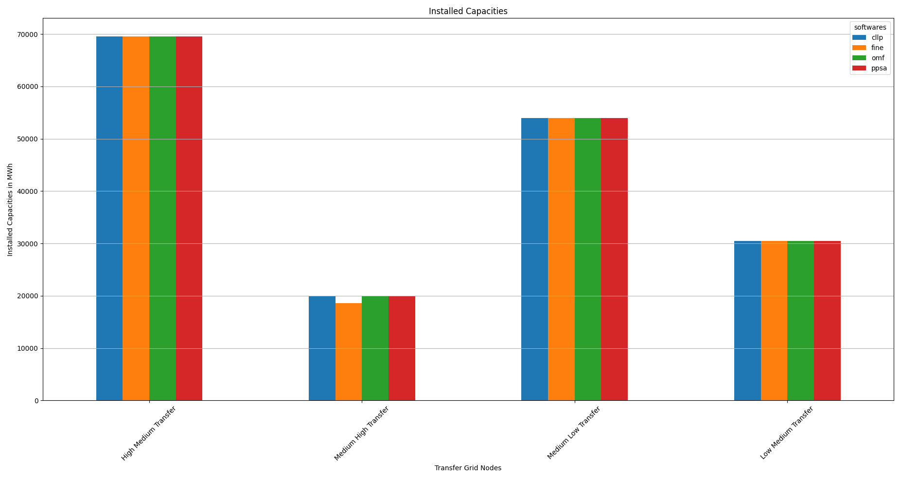
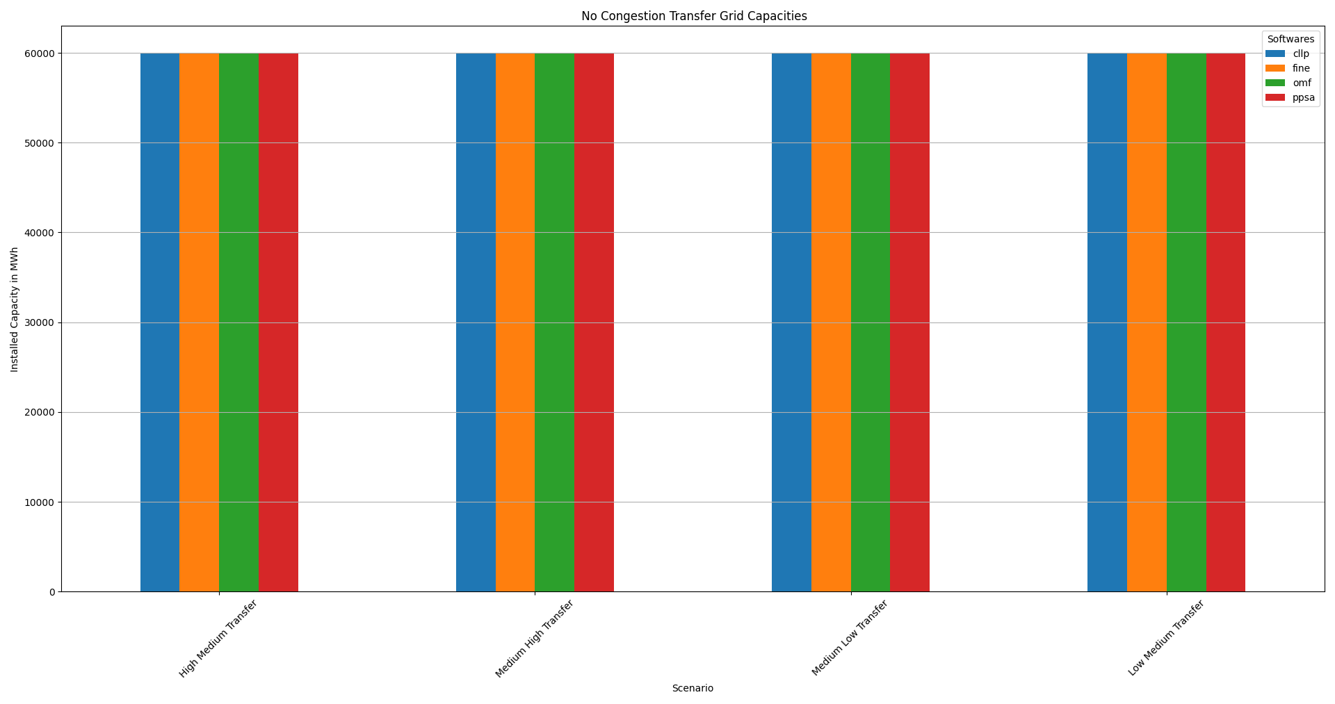
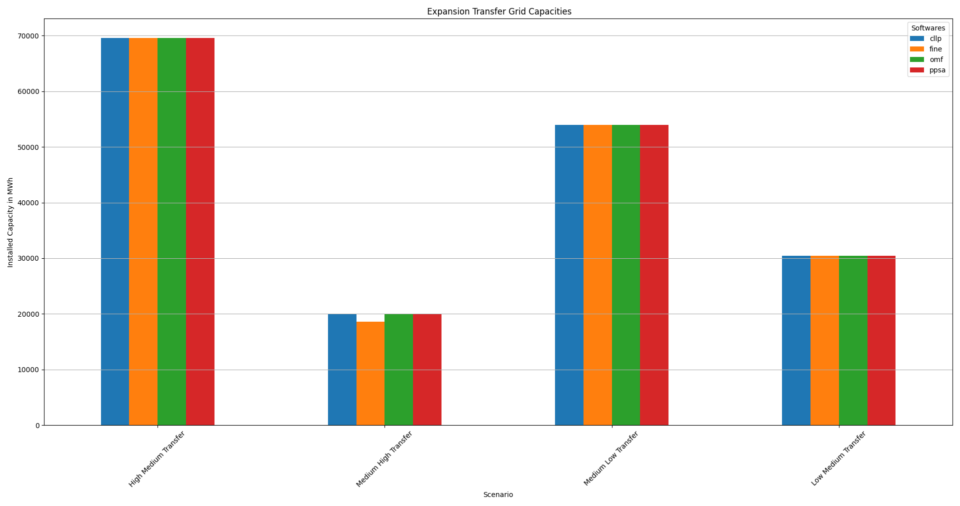
Transfer Grid Installed Capacity
Nodes |
cllp |
fine |
omf |
ppsa |
High Medium Transfer |
69567 |
69567 |
69567 |
69567 |
Medium High Transfer |
20000 |
18600 |
20000 |
19999 |
Medium Low Transfer |
53955 |
53955 |
53955 |
53955 |
Low Medium Transfer |
30432 |
30432 |
30432 |
30432 |
Medium Voltage Grid Loads Results
Comparing the integrated global results from above as well as the detailed numerical load results of the high, medium and low voltage grid busses, shows, that the different softwares all solve the TransC model-scenario-combination quite similarly.
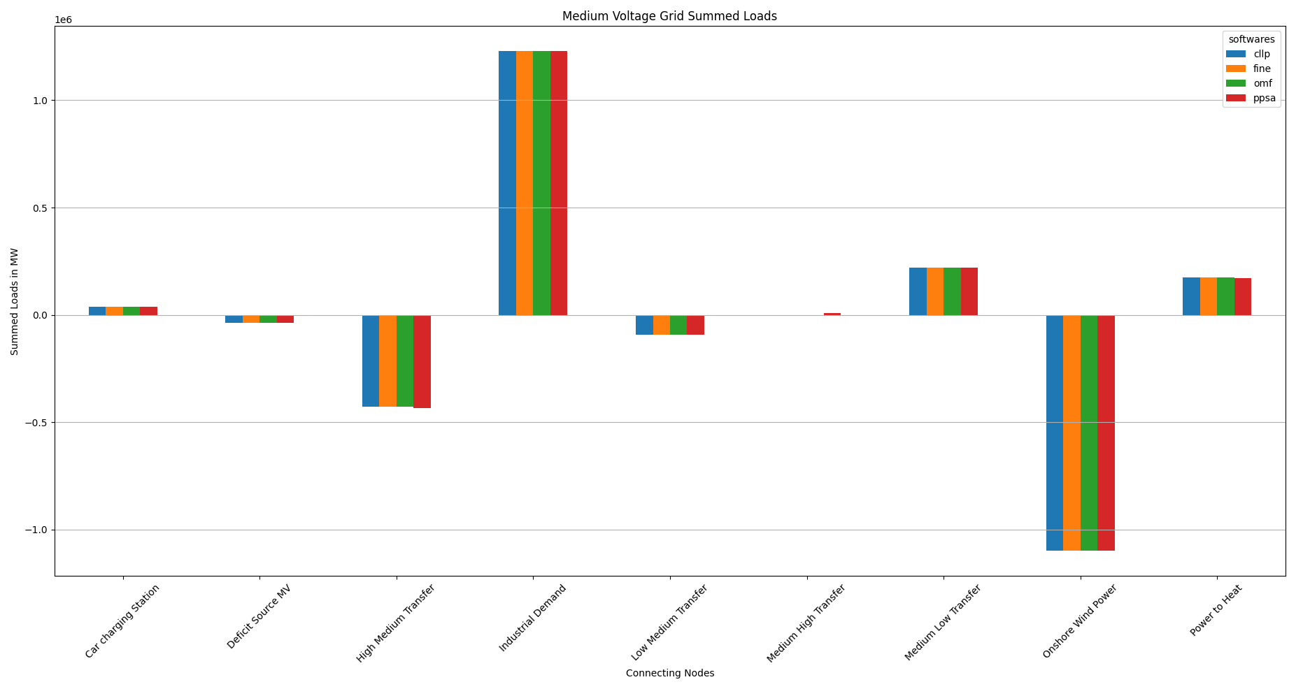
The representative summed loads bar plot as well as the load profile plot for software “oemof” are shown below.
Summed Loads
Load-Medium Voltage Grid [MW] |
cllp |
fine |
omf |
ppsa |
Car charging Station |
37026 |
37026 |
37026 |
37026 |
Deficit Source MV |
0 |
0 |
0 |
0 |
Excess Sink MV |
0 |
0 |
0 |
0 |
High Medium Transfer |
-877977 |
-877977 |
-877977 |
-877977 |
Industrial Demand |
1229008 |
1229008 |
1229008 |
1229008 |
Low Medium Transfer |
-103346 |
-103346 |
-103346 |
-103346 |
Medium High Transfer |
0 |
0 |
0 |
0 |
Medium Low Transfer |
673475 |
673475 |
673475 |
673475 |
Onshore Wind Power |
-1099866 |
-1099866 |
-1099866 |
-1099866 |
Power to Heat |
141680 |
141680 |
141680 |
141680 |
Inflows are negative, outflows positive. Connected zero-flow nodes are not shown:

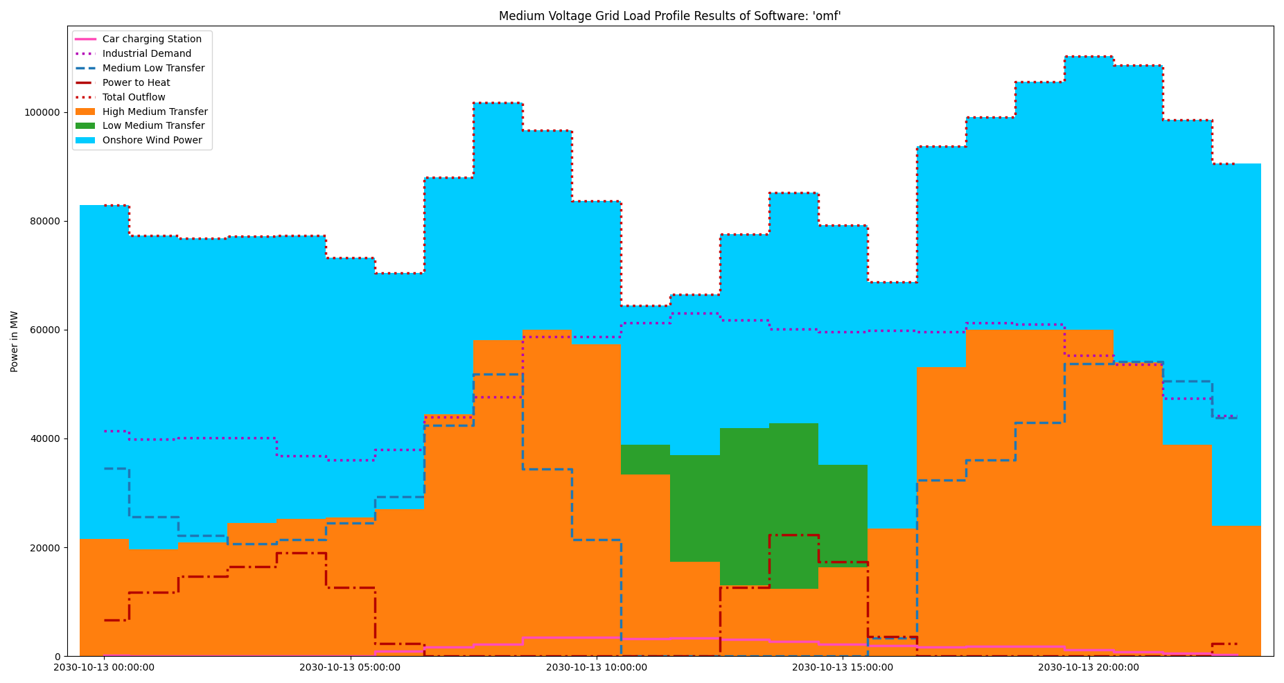
Load Profile Plot “Oemof”
Deficit Source MV |
High Medium Transfer |
Low Medium Transfer |
Onshore Wind Power |
Car charging Station |
Excess Sink MV |
Industrial Demand |
Medium High Transfer |
Medium Low Transfer |
Power to Heat |
|
2030-10-13 00:00:00 |
0 |
-21530.999 |
0.0 |
-61321.041 |
199.55034 |
0 |
41420.707 |
0 |
34579.956 |
6651.8273 |
2030-10-13 01:00:00 |
0 |
-19679.209 |
0.0 |
-57645.374 |
33.761407 |
0 |
39808.658 |
0 |
25675.673 |
11806.491 |
2030-10-13 02:00:00 |
0 |
-20854.971 |
0.0 |
-55988.777 |
23.179135 |
0 |
40077.333 |
0 |
22120.867 |
14622.369 |
2030-10-13 03:00:00 |
0 |
-24432.298 |
0.0 |
-52771.444 |
23.179135 |
0 |
40077.333 |
0 |
20636.279 |
16466.952 |
2030-10-13 04:00:00 |
0 |
-25190.678 |
0.0 |
-52130.374 |
79.617922 |
0 |
36853.235 |
0 |
21393.545 |
18994.654 |
2030-10-13 05:00:00 |
0 |
-25431.492 |
0.0 |
-47729.758 |
93.727619 |
0 |
36002.431 |
0 |
24427.32 |
12637.772 |
2030-10-13 06:00:00 |
0 |
-26990.02 |
0.0 |
-43383.064 |
912.09003 |
0 |
37927.934 |
0 |
29254.143 |
2278.9176 |
2030-10-13 07:00:00 |
0 |
-44435.758 |
0.0 |
-43520.864 |
1698.7056 |
0 |
43883.56 |
0 |
42374.356 |
0.0 |
2030-10-13 08:00:00 |
0 |
-58020.43 |
0.0 |
-43664.656 |
2192.545 |
0 |
47645.008 |
0 |
51847.533 |
0.0 |
2030-10-13 09:00:00 |
0 |
-67129.06 |
0.0 |
-36630.859 |
3473.0 |
0 |
58750.236 |
0 |
41536.684 |
0.0 |
2030-10-13 10:00:00 |
0 |
-57285.428 |
0.0 |
-26343.783 |
3444.7806 |
0 |
58750.236 |
0 |
21434.195 |
0.0 |
2030-10-13 11:00:00 |
0 |
-33327.749 |
-5472.3418 |
-25663.769 |
3250.7723 |
0 |
61213.088 |
0 |
0.0 |
0.0 |
2030-10-13 12:00:00 |
0 |
-17294.145 |
-19706.517 |
-29453.272 |
3360.1224 |
0 |
63093.812 |
0 |
0.0 |
0.0 |
2030-10-13 13:00:00 |
0 |
-13018.034 |
-28889.815 |
-35624.32 |
3134.3673 |
0 |
61750.438 |
0 |
0.0 |
12647.364 |
2030-10-13 14:00:00 |
0 |
-12406.164 |
-30432.837 |
-42280.663 |
2707.5489 |
0 |
60138.389 |
0 |
0.0 |
22273.726 |
2030-10-13 15:00:00 |
0 |
-16375.402 |
-18844.881 |
-44012.151 |
2234.8741 |
0 |
59601.039 |
0 |
0.0 |
17396.521 |
2030-10-13 16:00:00 |
0 |
-23472.995 |
0.0 |
-45315.261 |
2005.5915 |
0 |
59869.714 |
0 |
3319.4264 |
3593.5244 |
2030-10-13 17:00:00 |
0 |
-53098.587 |
0.0 |
-40621.071 |
1716.3428 |
0 |
59601.039 |
0 |
32402.276 |
0.0 |
2030-10-13 18:00:00 |
0 |
-67467.231 |
0.0 |
-39003.418 |
1758.6718 |
0 |
61213.088 |
0 |
43498.889 |
0.0 |
2030-10-13 19:00:00 |
0 |
-69567.123 |
0.0 |
-45599.848 |
1790.4187 |
0 |
60944.414 |
0 |
52432.139 |
0.0 |
2030-10-13 20:00:00 |
0 |
-64210.078 |
0.0 |
-50297.034 |
1233.0856 |
0 |
55257.462 |
0 |
58016.564 |
0.0 |
2030-10-13 21:00:00 |
0 |
-53983.53 |
0.0 |
-54613.772 |
859.17867 |
0 |
53600.634 |
0 |
54137.489 |
0.0 |
2030-10-13 22:00:00 |
0 |
-38829.106 |
0.0 |
-59652.462 |
509.96367 |
0 |
47376.333 |
0 |
50595.271 |
0.0 |
2030-10-13 23:00:00 |
0 |
-23947.329 |
0.0 |
-66599.384 |
291.26337 |
0 |
44152.235 |
0 |
43792.749 |
2310.4665 |
Inflows are represented as stacked bars, outflows as stacked step plots. Connected zero-flow nodes are not shown:
Redispatch
For the TransE combination no redispatch is needed.
Circulated Energy Transport
For the TransE combination no energy is circulated between
busses to reduce the amount of excess sink fed energy (which is costly).
Comparison
Costs

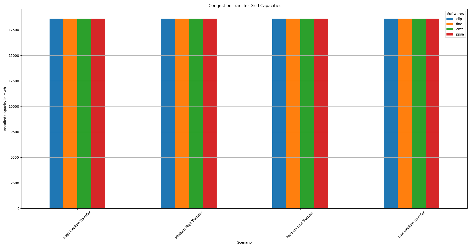
Installed Transfer Grid Capacities
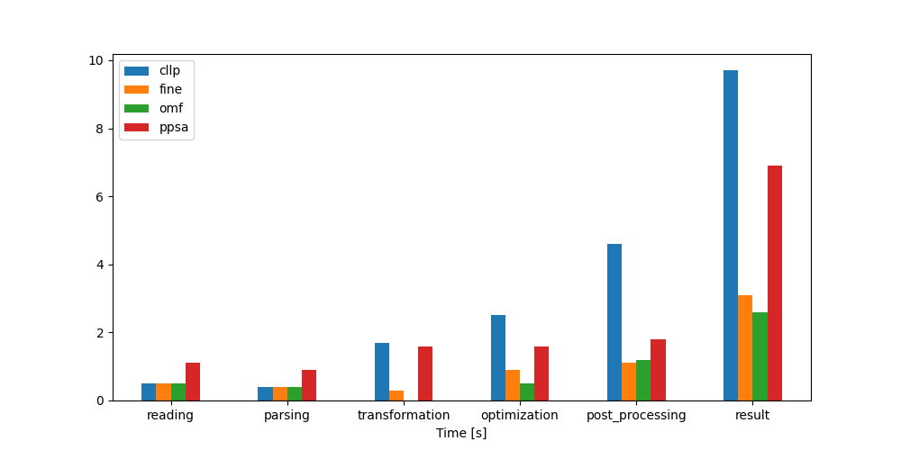
Computationel Ressources Used
Among the Trans combinations the Congestion scenario is the most time
intensive (if only slightly). Due to the relatively short timeframe optimized
transformation and post-processing constribute significantly to overall
ressources used.
Timing Results
Time [s] |
cllp |
fine |
omf |
ppsa |
reading |
0.5 |
0.5 |
0.5 |
1.1 |
parsing |
0.4 |
0.4 |
0.4 |
0.9 |
transformation |
1.7 |
0.3 |
0.0 |
1.6 |
optimization |
2.5 |
0.9 |
0.5 |
1.6 |
post_processing |
4.6 |
1.1 |
1.2 |
1.8 |
result |
9.7 |
3.1 |
2.6 |
6.9 |
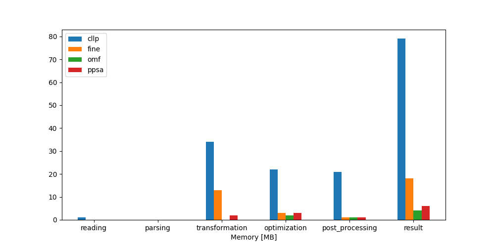
Memory Results
Memory [MB] |
cllp |
fine |
omf |
ppsa |
reading |
1.0 |
0.0 |
0.0 |
0.0 |
parsing |
0.0 |
0.0 |
0.0 |
0.0 |
transformation |
34.0 |
13.0 |
0.0 |
2.0 |
optimization |
22.0 |
3.0 |
2.0 |
3.0 |
post_processing |
21.0 |
1.0 |
1.0 |
1.0 |
result |
79.0 |
18.0 |
4.0 |
6.0 |
Advanced Graphs
Following sections show the advanced graph representations of the three
model-scenario-combinations investigated. Since result variation in between
softwares compared is low, only the Oemof graph is shown.
No Congestion Commitment

Congestion Commitment

Expansion

Key Observations
Comparing the above advanced graph visulaizations, three main differences are easily observed between the three scenarios:
Inside the
Commitment - congestionscenario the high to medium transfer line is used to full capacityIn comparison to the other two
Transscenarios, the low voltage deficit source is used in theCommitment - congestionscenario:In the
Expansionscenario the is overall less expensive to expand high to medium and medium to high transfer capacities and utilize the high voltage connected coal fired power plant in comparison the bio gas fired low voltage connected cogeneration plant (BHKW)
Key Conclusions
The Key Goal could be served in the sense of developing a reference supply system model in conjunction with two relevant and contemporary scenario formulations to test out the modelling softwares
Calliope,Fine,OemofandPypsa.All of the 4 aims (Thesis-> Method -> Modelling -> MSC Selection ) formulated, with regards to component focused model behaviour, were successfully addressed:
Modelling energy transportation losses and maximum transferable energy in grid-like components:
The component-combination
High Medium Transfer/Medium High TransferandMedium Low Transfer/Low Medium Transferrepresent electrical energy transport components able to model flow rate dependend losses in form of an efficiency value as well as a maximum flow rate via installed capacity as discussed in detail in Hanke, Ammon in subsections 3.8.5 to 3.8.8
Modelling grid congestion issues:
Restricting installed transfer capacity to 20000MW in the Congestion Commitment Scenario leads to an optimal solution more expensive than without restrictions, as can be seen in Integrated Global Results. Fully utilizing transport capacities while requiring the low voltage deficit source to componesate as show by the Advanced Graphs (and the subsequent Key Observations).
Modelling congestion issue related redispatch:
By limiting the transfer capacity to 20000MW in the Congestion Commitment Scenario a redispatch in power generation from high voltage to the medium voltage grid becomes necessary as observable in figure Load Profile Plot “Oemof” and lsited in table Redispatch.
Potential expansion of transportation capacities to avoid two and three.
In addition to that following insights were gained with regards to the softwares used:
Given the same input it is possible, but not necessarily directly implied, to produce the exact same results on relatively large and complex energy supply system models for all softwares investigated. Also and in particular when modelling grid like structures with the help of two tessif transformer components, as desmonstrated.
Using two tessif transformer components in conjunction with an excess sink and deficit source allows modelling required redispatch efficiently. It also ensures the solver can find an optimal solution by providing unlimited albeit expensive energy in- and output.
As seen in the Integrated Global Results, emission allocation differs between softwares. If however neither storage nore connector components are used in conjunction with allocated emissions, deviation is relatively small. In addtion, if the investigated scenario does not impose an emission limit, as in the above scenarios, no subsequent result variation are observed.
The benefits of Tessif facilitating energy supply system model creation, transformation, optimization, post-processing, result comparison and visualization again become observable when inspecting the programming code with which the above results were generated.
On comparitevly small optimization timeframes like the above 24 hourly steps Tessif introduced need of computational ressources is significant It therfor has to be taken into account in cases where a lot of these small optimizations are to be performed in parallel.
Comparing the computational ressourcess needed between softwares on the above model-scenario-combinations, it seems as though tessif-oemof is generally more efficient than tessif-fine, which is more efficient than tessif-pypsa, which in turn is more efficient than tessif-calliope.