Minimum Working Examples

create_mwe	Create a minimum working example using pypsa.
emission_objective	Create a minimum working example using pypsa.
create_transshipment_problem	Create a transshipment problem.
create_storage_example	Create a small energy system utilizing a storage using pypsa.
create_transformer_example	Create a small energy system utiulizing an electrical power transformer using pypsa.
create_chp_example	Create a combined heat and power example using pypsa.
create_component_scenario	Create a model of a generic component based energy system using pypsa.

py_hard

py_hard is a tessif module for giving examples on how to create a pypsa energy system It collects minimum working examples, meaningful working examples and full fledged use case wrappers for common scenarios.

tessif.examples.data.pypsa.py_hard.create_mwe(directory=None)

Create a minimum working example using pypsa.

Creates a simple energy system simulation to potentially store it on disc in directory as filename

Parameters:

directory (str, default=None) –

String representing of the path the created energy system is stored in. Passed to pypsa.Network.export_to_csv_folder().

If set to None (default) tessif.frused.paths.write_dir/pypsa/mwe will be the chosen directory.

Returns:

optimized_es – Energy system carrying the optimization results.

Return type:

Network

Examples

Using create_mwe() to quickly access a tessif energy system to use for doctesting, or trying out this frameworks utilities.

(For a step by step explanation see Minimum Working Example):

>>> import tessif.examples.data.pypsa.py_hard as pypsa_coded_examples
>>> import sys
>>> pypsa_es = pypsa_coded_examples.create_mwe()

Show the exported directory’s content:

>>> import os
>>> from tessif.frused.paths import write_dir
>>> for fle in sorted(os.listdir(os.path.join(write_dir, 'pypsa', 'mwe'))):
...     print(fle)
buses-marginal_price.csv
buses.csv
generators-p.csv
generators-p_max_pu.csv
generators.csv
investment_periods.csv
loads-p.csv
loads.csv
network.csv
snapshots.csv

tessif.examples.data.pypsa.py_hard.emission_objective(directory=None)

Create a minimum working example using pypsa.

Optimizing it for costs and keeping the total emissions below an emission objective.

Parameters:

directory (str, default=None) –

String representing of the path the created energy system is stored in. Passed to pypsa.Network.export_to_csv_folder().

If set to None (default) tessif.frused.paths.write_dir/pypsa/emission_objective will be the chosen directory.

Returns:

optimized_es – Energy system carrying the optimization results.

Return type:

Network

Examples

Using emission_objective() to quickly access an optimized pypsa energy system to use for doctesting, or trying out this frameworks utilities.

(For a step by step explanation on how to create an oemof minimum working example see Minimum Working Example):

>>> import tessif.examples.data.pypsa.py_hard as coded_examples
>>> optimized_es = coded_examples.emission_objective()

Show the emission constraint:

>>> import pprint
>>> pprint.pprint(optimized_es.global_constraints)
attribute            type  investment_period carrier_attribute sense  constant   mu
name
co2_limit  primary_energy                NaN     co2_emissions    <=      30.0  3.0

Note how utilizing the generator is cheaper, but due to the emission constraint the renewable is used during the last timestep:

>>> print(optimized_es.generators_t.p)
name                 Renewable  Gas Generator
snapshot
1990-07-13 00:00:00        0.0           10.0
1990-07-13 01:00:00        0.0           10.0
1990-07-13 02:00:00        0.0           10.0
1990-07-13 03:00:00       10.0            0.0

See user’s guide on Secondary Objectives for more on this example.

tessif.examples.data.pypsa.py_hard.create_transshipment_problem(directory=None)

Create a transshipment problem. using pypsa.

Optimizing it for costs.

Parameters:

directory (str, default=None) –

String representing of the path the created energy system is stored in. Passed to pypsa.Network.export_to_csv_folder().

If set to None (default) tessif.frused.paths.write_dir/pypsa/transshipment will be the chosen directory.

Returns:

optimized_es – Energy system carrying the optimization results.

Return type:

Network

Examples

Using create_transshipment_problem() to quickly access an optimized pypsa energy system to use for doctesting, or trying out this frameworks utilities.

(For a step by step explanation see Minimum Working Example):

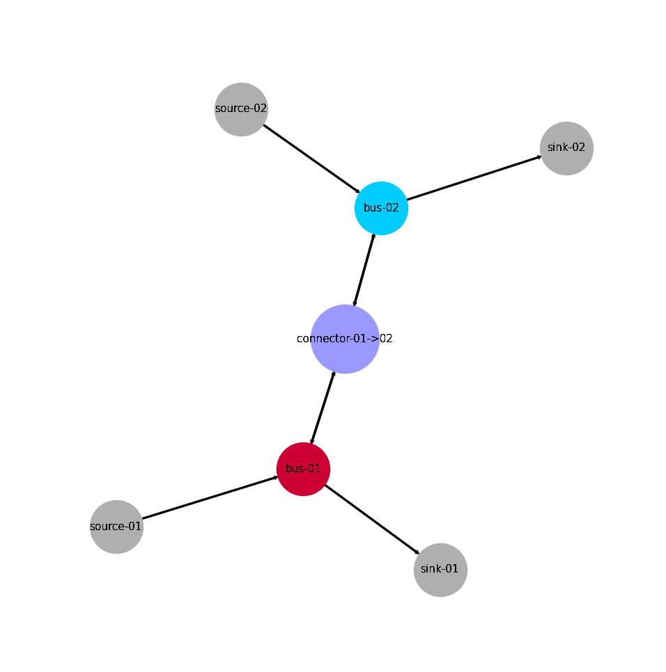
>>> import tessif.examples.data.pypsa.py_hard as coded_pypsa_examples
>>> pypsa_es = coded_pypsa_examples.create_transshipment_problem()
>>> for link in pypsa_es.links.index:
...     print(link)
connector-01->02

>>> import tessif.transform.es2mapping.ppsa as post_process_pypsa
>>> resultier = post_process_pypsa.LoadResultier(pypsa_es)

>>> print(resultier.node_load['connector-01->02'])
connector-01->02     bus-01  bus-02  bus-01  bus-02
1990-07-13 00:00:00   -10.0    -0.0     0.0    10.0
1990-07-13 01:00:00    -0.0    -5.0     5.0     0.0
1990-07-13 02:00:00    -0.0    -0.0     0.0     0.0

>>> print(resultier.node_load['bus-01'])
bus-01               connector-01->02  source-01  connector-01->02  sink-01
1990-07-13 00:00:00              -0.0      -10.0              10.0      0.0
1990-07-13 01:00:00              -5.0      -10.0               0.0     15.0
1990-07-13 02:00:00              -0.0      -10.0               0.0     10.0

>>> print(resultier.node_load['bus-02'])
bus-02               connector-01->02  source-02  connector-01->02  sink-02
1990-07-13 00:00:00             -10.0       -5.0               0.0     15.0
1990-07-13 01:00:00              -0.0       -5.0               5.0      0.0
1990-07-13 02:00:00              -0.0      -10.0               0.0     10.0

Visualize the energy system for better understanding what the output means:

>>> import matplotlib.pyplot as plt
>>> import tessif.visualize.nxgrph as nxv
>>> import tessif.transform.nxgrph as nxt
>>> grph = nxt.Graph(resultier)
>>> drawing_data = nxv.draw_graph(
...     grph,
...     node_color={'connector-01->02': '#9999ff',
...                 'bus-01': '#cc0033',
...                 'bus-02': '#00ccff'},
...     node_size={'connector': 5000},
...     layout='neato')
>>> # plt.show()  # commented out for simpler doctesting

tessif.examples.data.pypsa.py_hard.create_storage_example(directory=None)

Create a small energy system utilizing a storage using pypsa.

Optimizing it for costs.

Parameters:

directory (str, default=None) –

String representing of the path the created energy system is stored in. Passed to pypsa.Network.export_to_csv_folder().

If set to None (default) tessif.frused.paths.write_dir/pypsa/storage will be the chosen directory.

Returns:

optimized_es – Energy system carrying the optimization results.

Return type:

Network

Examples

Using create_storage_example() to quickly access an optimized pypsa energy system to use for doctesting, or trying out this frameworks utilities.

(For a step by step explanation see Minimum Working Example):

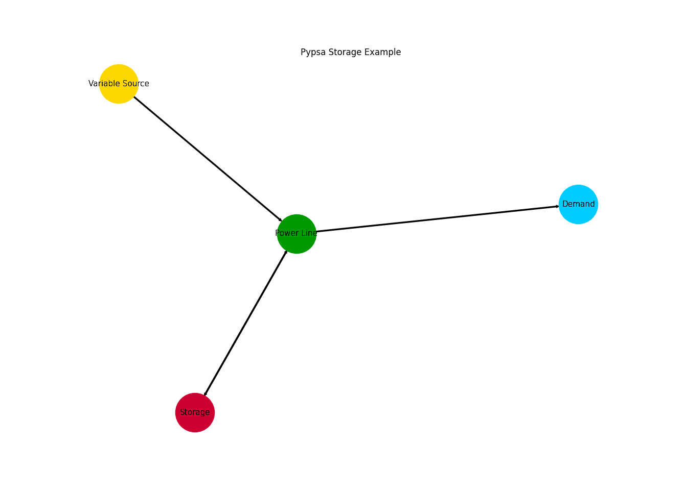
>>> # import the storage example and optimize it:
>>> import tessif.examples.data.pypsa.py_hard as coded_pypsa_examples
>>> pypsa_es = coded_pypsa_examples.create_storage_example()
>>> for storage in pypsa_es.storage_units.index:
...     print(storage)
Storage

>>> # import the post processing utility:
>>> import tessif.transform.es2mapping.ppsa as post_process_pypsa

>>> # use it to get the  load results:
>>> resultier = post_process_pypsa.LoadResultier(pypsa_es)
>>> for load in resultier.node_load.values():
...     print(load)
Variable Source      Power Line
1990-07-13 00:00:00        19.0
1990-07-13 01:00:00        19.0
1990-07-13 02:00:00        19.0
1990-07-13 03:00:00         0.0
1990-07-13 04:00:00         0.0
Demand               Power Line
1990-07-13 00:00:00       -10.0
1990-07-13 01:00:00       -10.0
1990-07-13 02:00:00        -7.0
1990-07-13 03:00:00       -10.0
1990-07-13 04:00:00       -10.0
Storage              Power Line  Power Line
1990-07-13 00:00:00        -9.0         0.0
1990-07-13 01:00:00        -9.0         0.0
1990-07-13 02:00:00       -12.0         0.0
1990-07-13 03:00:00        -0.0        10.0
1990-07-13 04:00:00        -0.0        10.0
Power Line           Storage  Variable Source  Demand  Storage
1990-07-13 00:00:00     -0.0            -19.0    10.0      9.0
1990-07-13 01:00:00     -0.0            -19.0    10.0      9.0
1990-07-13 02:00:00     -0.0            -19.0     7.0     12.0
1990-07-13 03:00:00    -10.0             -0.0    10.0      0.0
1990-07-13 04:00:00    -10.0             -0.0    10.0      0.0

>>> # use it to get the storage soc results:
>>> resultier = post_process_pypsa.StorageResultier(pypsa_es)
>>> print(resultier.node_soc['Storage'])
1990-07-13 00:00:00     9.0
1990-07-13 01:00:00    18.0
1990-07-13 02:00:00    30.0
1990-07-13 03:00:00    20.0
1990-07-13 04:00:00    10.0
Freq: H, Name: Storage, dtype: float64

>>> # use it to get the storage capacity and characteristic value results:
>>> resultier = post_process_pypsa.CapacityResultier(pypsa_es)
>>> # capacity results:
>>> for node, capacity in resultier.node_installed_capacity.items():
...     print(f'{node}: {capacity}')
Power Line: None
Variable Source: 19.0
Demand: 10.0
Storage: 30.0

>>> # characteristic value results:
>>> for node, cv in resultier.node_characteristic_value.items():
...     if cv is not None:
...         cv = round(cv, 2)
...     print(f'{node}: {cv}')
Power Line: None
Variable Source: 0.6
Demand: 0.94
Storage: 0.58

Visualize the energy system for better understanding what the output means:

>>> import matplotlib.pyplot as plt
>>> import tessif.visualize.nxgrph as nxv
>>> import tessif.transform.nxgrph as nxt
>>> grph = nxt.Graph(resultier)
>>> drawing_data = nxv.draw_graph(
...     grph,
...     node_color={'Power Line': '#009900',
...                 'Storage': '#cc0033',
...                 'Demand': '#00ccff',
...                 'Variable Source': '#ffD700',},
...     layout='neato')
>>> # plt.show()  # commented out for simpler doctesting

tessif.examples.data.pypsa.py_hard.create_transformer_example(directory=None)

Create a small energy system utiulizing an electrical power transformer using pypsa.

Optimizing it for costs.

Parameters:

directory (str, default=None) –

String representing of the path the created energy system is stored in. Passed to pypsa.Network.export_to_csv_folder().

If set to None (default) tessif.frused.paths.write_dir/pypsa/transformer will be the chosen directory.

Returns:

optimized_es – Energy system carrying the optimization results.

Return type:

Network

Examples

Using create_transformer_example() to quickly access an optimized pypsa energy system to use for doctesting, or trying out this frameworks utilities.

(For a step by step explanation see Minimum Working Example):

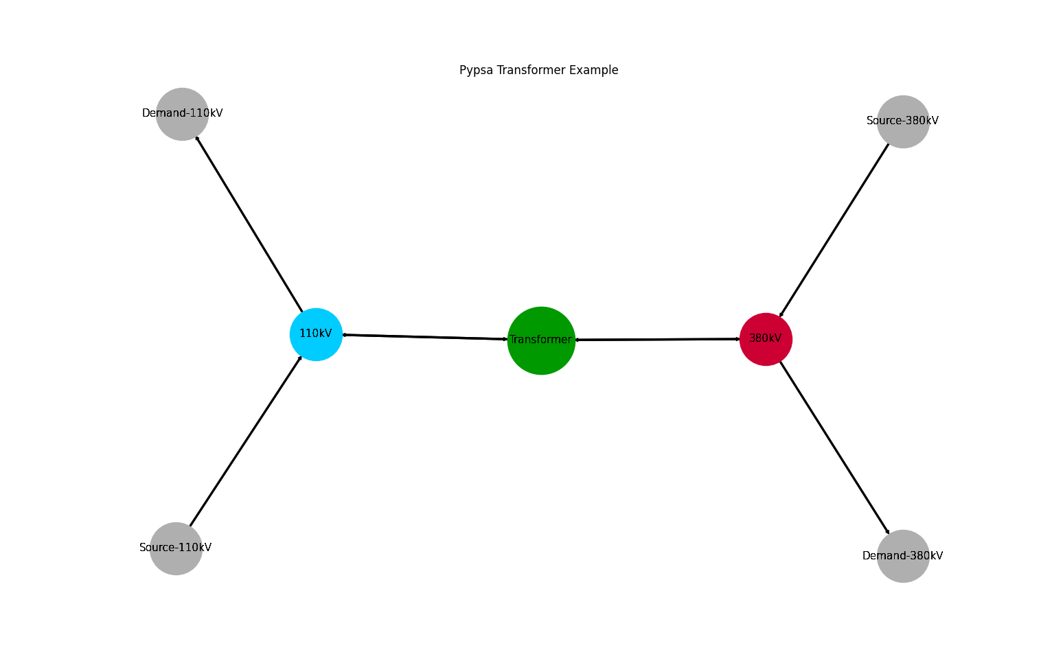
>>> # import the transformer example and optimize it:
>>> import tessif.examples.data.pypsa.py_hard as coded_pypsa_examples
>>> pypsa_es = coded_pypsa_examples.create_transformer_example()
>>> for transformer in pypsa_es.transformers.index:
...     print(transformer)
Transformer

>>> # import the post processing utility:
>>> import tessif.transform.es2mapping.ppsa as post_process_pypsa

>>> # use it to get the  load results:
>>> resultier = post_process_pypsa.LoadResultier(pypsa_es)
>>> for load in resultier.node_load.values():
...     print(load)
...     print()
Source-380kV         380kV
1990-07-13 00:00:00   20.0
1990-07-13 01:00:00   20.0
1990-07-13 02:00:00    0.0
1990-07-13 03:00:00    0.0

Source-110kV         110kV
1990-07-13 00:00:00    0.0
1990-07-13 01:00:00    0.0
1990-07-13 02:00:00   20.0
1990-07-13 03:00:00   20.0

Demand-380kV         380kV
1990-07-13 00:00:00  -10.0
1990-07-13 01:00:00  -10.0
1990-07-13 02:00:00  -10.0
1990-07-13 03:00:00  -10.0

Demand-110kV         110kV
1990-07-13 00:00:00  -10.0
1990-07-13 01:00:00  -10.0
1990-07-13 02:00:00  -10.0
1990-07-13 03:00:00  -10.0

Transformer          110kV  380kV  110kV  380kV
1990-07-13 00:00:00   -0.0  -10.0   10.0    0.0
1990-07-13 01:00:00   -0.0  -10.0   10.0    0.0
1990-07-13 02:00:00  -10.0   -0.0    0.0   10.0
1990-07-13 03:00:00  -10.0   -0.0    0.0   10.0

380kV                Source-380kV  Transformer  Demand-380kV  Transformer
1990-07-13 00:00:00         -20.0         -0.0          10.0         10.0
1990-07-13 01:00:00         -20.0         -0.0          10.0         10.0
1990-07-13 02:00:00          -0.0        -10.0          10.0          0.0
1990-07-13 03:00:00          -0.0        -10.0          10.0          0.0

110kV                Source-110kV  Transformer  Demand-110kV  Transformer
1990-07-13 00:00:00          -0.0        -10.0          10.0          0.0
1990-07-13 01:00:00          -0.0        -10.0          10.0          0.0
1990-07-13 02:00:00         -20.0         -0.0          10.0         10.0
1990-07-13 03:00:00         -20.0         -0.0          10.0         10.0

>>> # use it to get the storage capacity and characteristic value results:
>>> resultier = post_process_pypsa.CapacityResultier(pypsa_es)
>>> # capacity results:
>>> for node, capacity in resultier.node_installed_capacity.items():
...     print(f'{node}: {capacity}')
380kV: None
110kV: None
Source-380kV: 20.0
Source-110kV: 20.0
Demand-380kV: 10.0
Demand-110kV: 10.0
Transformer: 160.0

>>> # characteristic value results:
>>> for node, cv in resultier.node_characteristic_value.items():
...     if cv is not None:
...         cv = round(cv, 2)
...     print(f'{node}: {cv}')
380kV: None
110kV: None
Source-380kV: 0.5
Source-110kV: 0.5
Demand-380kV: 1.0
Demand-110kV: 1.0
Transformer: 0.06

Visualize the energy system for better understanding what the output means:

>>> import matplotlib.pyplot as plt
>>> import tessif.visualize.nxgrph as nxv
>>> import tessif.transform.nxgrph as nxt
>>> grph = nxt.Graph(resultier)
>>> drawing_data = nxv.draw_graph(
...     grph,
...     node_color={'Transformer': '#9999ff',
...                 '380kV': '#cc0033',
...                 '110kV': '#00ccff'},
...     node_size={'Transformer': 5000},
...     layout='neato')
>>> # plt.show()  # commented out for simpler doctesting

tessif.examples.data.pypsa.py_hard.create_chp_example(directory=None)

Create a combined heat and power example using pypsa.

Creates a simple energy system simulation to potentially store it on disc in directory.

Warning

For tessif's post processing to work as intended a pypsa link intendend to be used as a Transformer some default behaviour has to be overriden. Refer to the source code of this example as well as the pypsa chp example

Parameters:

directory (str, default=None) –

String representing of the path the created energy system is stored in. Passed to pypsa.Network.export_to_csv_folder().

If set to None (default) tessif.frused.paths.write_dir/pypsa/chp will be the chosen directory.

Returns:

optimized_es – Energy system carrying the optimization results.

Return type:

Network

Examples

Using create_chp() to quickly access a tessif energy system to use for doctesting, or trying out this frameworks utilities.

(For a step by step explanation see Minimum Working Example):

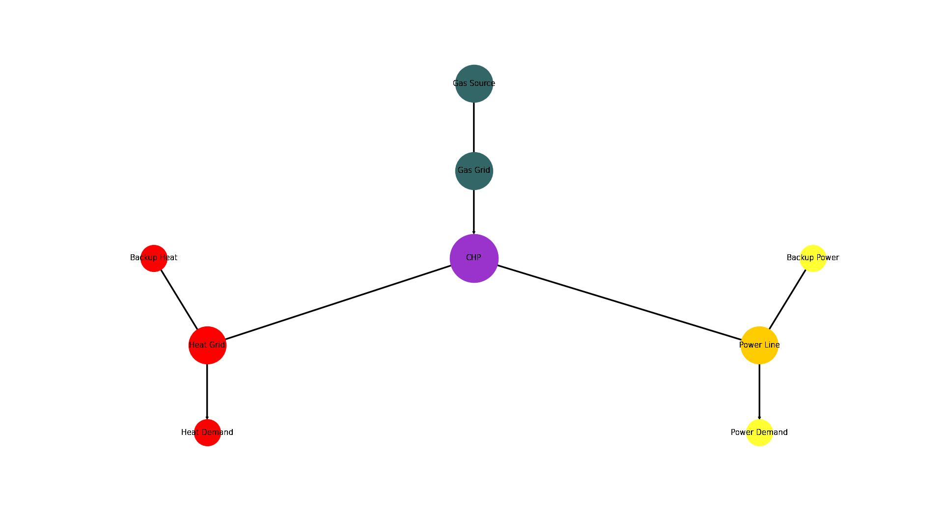
>>> import tessif.examples.data.pypsa.py_hard as pypsa_coded_examples
>>> import sys
>>> pypsa_es = pypsa_coded_examples.create_chp_example()

Do some post processing and show the results:

>>> import tessif.transform.es2mapping.ppsa as post_process_pypsa
>>> resultier = post_process_pypsa.LoadResultier(pypsa_es)

>>> print(resultier.node_load['CHP'])
CHP                  Gas Grid  Heat Grid  Power Line
1990-07-13 00:00:00     -20.0       10.0         6.0
1990-07-13 01:00:00     -20.0       10.0         6.0

>>> print(resultier.node_load['Heat Grid'])
Heat Grid            Backup Heat   CHP  Heat Demand
1990-07-13 00:00:00         -0.0 -10.0         10.0
1990-07-13 01:00:00         -0.0 -10.0         10.0

>>> print(resultier.node_load['Power Line'])
Power Line           Backup Power  CHP  Power Demand
1990-07-13 00:00:00          -4.0 -6.0          10.0
1990-07-13 01:00:00          -4.0 -6.0          10.0

Generate a visual representation of the energy system:

>>> import matplotlib.pyplot as plt
>>> import tessif.visualize.nxgrph as nxv
>>> import tessif.transform.nxgrph as nxt

>>> grph = nxt.Graph(resultier)
>>> formatier = post_process_pypsa.NodeFormatier(pypsa_es, cgrp='name')

>>> drawing_data = nxv.draw_graph(
...     grph,
...     formatier=formatier,
...     node_size={'CHP': 5000},
... )
>>> # plt.show()  # commented out for simpler doctesting

tessif.examples.data.pypsa.py_hard.create_component_scenario(expansion_problem=False, periods=3, directory=None)

Create a model of a generic component based energy system using pypsa.

Parameters:

• expansion_problem (bool, default=False) – Boolean which states whether a commitment problem (False) or expansion problem (True) is to be solved

• periods (int, default=3) – Number of time steps of the evaluated timeframe (one time step is one hour)

• directory (str, default=None) –

  String representing of the path the created energy system is stored in. Passed to pypsa.Network.export_to_csv_folder().

  If set to None (default) tessif.frused.paths.write_dir/pypsa/component will be the chosen directory.

Returns:

optimized_es – Energy system carrying the optimization results.

Return type:

Network

Examples

Using create_component_scenario() to quickly access a pypsa energy system to use for doctesting, or trying out this frameworks utilities.

(For a step by step explanation see Minimum Working Example):

>>> import tessif.examples.data.pypsa.py_hard as pypsa_coded_examples
>>> pypsa_es = pypsa_coded_examples.create_component_scenario()